Visualize and bring together data from the SAIL campaign and NOAA

When reading and analyzing data, its is useful to bring together data from different organizations. This not only expands the data available for scientists and their research, but is also useful for quality controls checks. In this notebook, we look at both the datasets produce by ARM instruments in the SAIL campaign as well as instruments provided by NOAA at their KPS site near the SAIL campaign location.

Imports

# Import our modules
import datetime as dt
import glob


import matplotlib
import matplotlib.pyplot as plt
import numpy as np
import xarray as xr

import act

Download and visualize our data using ACT

# Download the NOAA KPS site files from 22:00 and 23:00
result_22_kps = act.discovery.download_noaa_psl_data(
    site='kps', instrument='Radar FMCW Moment', startdate='20220801', hour='22'
)
result_23_kps = act.discovery.download_noaa_psl_data(
    site='kps', instrument='Radar FMCW Moment', startdate='20220801', hour='23'
)

Downloading dkps2221322a.mom
Downloading hkps2221322a.mom
Downloading kps2221322.raw
Downloading dkps2221323a.mom
Downloading hkps2221323a.mom
Downloading kps2221323.raw

# Read in the .raw file.  Spectra data are also downloaded
ds1_kps = act.io.noaapsl.read_psl_radar_fmcw_moment([result_22_kps[-1], result_23_kps[-1]])

# Read in the parsivel files from NOAA's webpage.
url = [
    'https://downloads.psl.noaa.gov/psd2/data/realtime/DisdrometerParsivel/Stats/kps/2022/213/kps2221322_stats.txt',
    'https://downloads.psl.noaa.gov/psd2/data/realtime/DisdrometerParsivel/Stats/kps/2022/213/kps2221323_stats.txt',
]
ds2_kps = act.io.noaapsl.read_psl_parsivel(url)

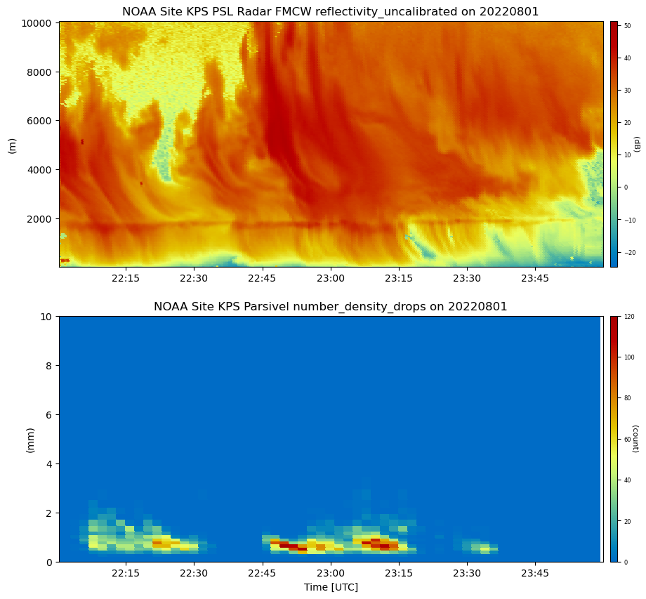
# First we plot the NOAA FMCW and parsivel from the KPS site

# Create display object with both datasets
display = act.plotting.TimeSeriesDisplay(
    {"NOAA Site KPS PSL Radar FMCW": kps_ds1, "NOAA Site KPS Parsivel": kps_ds2},
    subplot_shape=(2,),
    figsize=(10, 10),
)

# Plot the subplots
display.plot(
    'reflectivity_uncalibrated',
    dsname='NOAA Site KPS PSL Radar FMCW',
    cmap='act_HomeyerRainbow',
    subplot_index=(0,),
)
display.plot(
    'number_density_drops',
    dsname='NOAA Site KPS Parsivel',
    cmap='act_HomeyerRainbow',
    subplot_index=(1,),
)
# Set limits
display.axes[1].set_ylim([0, 10])
plt.show()

Create a Multipanel Plot to Compare the KAZR and Parsivel

# Use arm username and token to retrieve files.
# This is commented out as the files have already been downloaded.

# token = 'arm_token'
# username = 'arm_username'

# Specify datastream and date range for KAZR data
ds_kazr = 'guckazrcfrgeM1.a1'
startdate = '2022-08-01'
enddate = '2022-08-01'

# Data already retrieved, but showing code below on how to download the files.
# act.discovery.download_data(username, token, ds_kazr, startdate, enddate)

# Index last 2 files for the 22:00 and 23:00 timeframe.
kazr_files = glob.glob(''.join(['./', ds_kazr, '/*nc']))
kazr_files[-2:]
kazr_ds = act.io.arm.read_arm_netcdf(kazr_files[-2:])

# Specify datastream and date range for KAZR data
ds_ld = 'gucldM1.b1'
startdate = '2022-08-01'
enddate = '2022-08-01'

# Data already retrieved, but showing code below on how to download the files.
# act.discovery.download_data(username, token, ds_ld, startdate, enddate)

# Index last 2 files for the 22:00 and 23:00 timeframe.
ld_files = glob.glob(''.join(['./', ds_ld, '/*cdf']))
ld_ds = act.io.arm.read_arm_netcdf(ld_files[0])

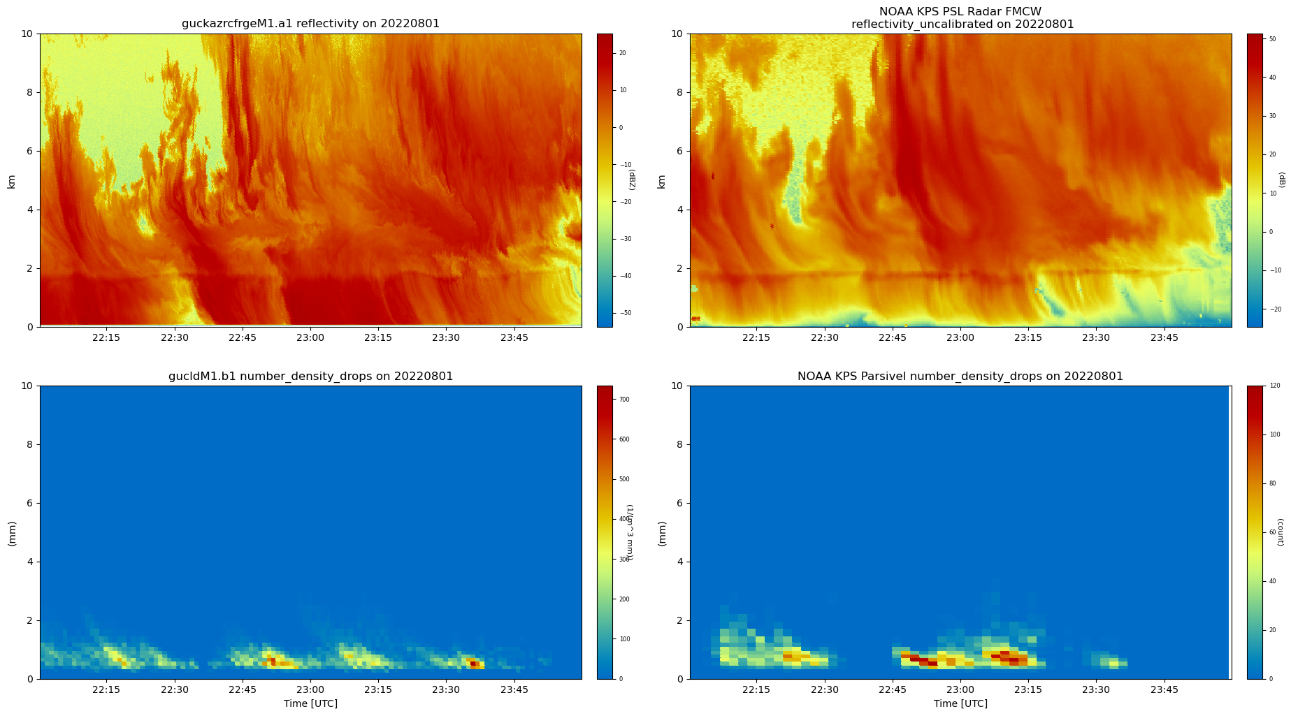
# We now want to plot and compare ARM and NOAA's instruments.

# Create a series display with all 4 datasets
display = act.plotting.TimeSeriesDisplay(
    {
        "NOAA KPS PSL Radar FMCW": kps_ds1,
        "NOAA KPS Parsivel": kps_ds2,
        "guckazrcfrgeM1.a1": kazr_ds,
        'gucldM1.b1': ld_ds,
    },
    subplot_shape=(2, 2),
    figsize=(22, 12),
)

# Set custom 2 line title for space
title = "NOAA KPS PSL Radar FMCW\n reflectivity_uncalibrated on 20220801"

# Plot the four subplots
display.plot(
    'reflectivity_uncalibrated',
    dsname='NOAA KPS PSL Radar FMCW',
    cmap='act_HomeyerRainbow',
    set_title=title,
    subplot_index=(0, 1),
)
display.plot(
    'number_density_drops',
    dsname='NOAA KPS Parsivel',
    cmap='act_HomeyerRainbow',
    subplot_index=(1, 1),
)
display.plot(
    'reflectivity', dsname='guckazrcfrgeM1.a1', cmap='act_HomeyerRainbow', subplot_index=(0, 0)
)
display.plot(
    'number_density_drops', dsname='gucldM1.b1', cmap='act_HomeyerRainbow', subplot_index=(1, 0)
)

# Update limits
display.axes[1, 0].set_ylim([0, 10])

display.axes[1, 1].set_ylim([0, 10])


display.axes[0, 0].set_ylim([0, 10000])
display.axes[0, 0].set_yticklabels(['0', '2', '4', '6', '8', '10'])
display.axes[0, 0].set_ylabel('km')

display.axes[0, 1].set_ylim([0, 10000])
display.axes[0, 1].set_yticklabels(['0', '2', '4', '6', '8', '10'])
display.axes[0, 1].set_ylabel('km')

plt.show()

C:\Users\sherm\AppData\Local\Temp\ipykernel_10268\1307396719.py:29: UserWarning: FixedFormatter should only be used together with FixedLocator
  display.axes[0, 0].set_yticklabels(['0', '2', '4','6', '8', '10'])
C:\Users\sherm\AppData\Local\Temp\ipykernel_10268\1307396719.py:33: UserWarning: FixedFormatter should only be used together with FixedLocator
  display.axes[0, 1].set_yticklabels(['0', '2', '4','6', '8', '10'])

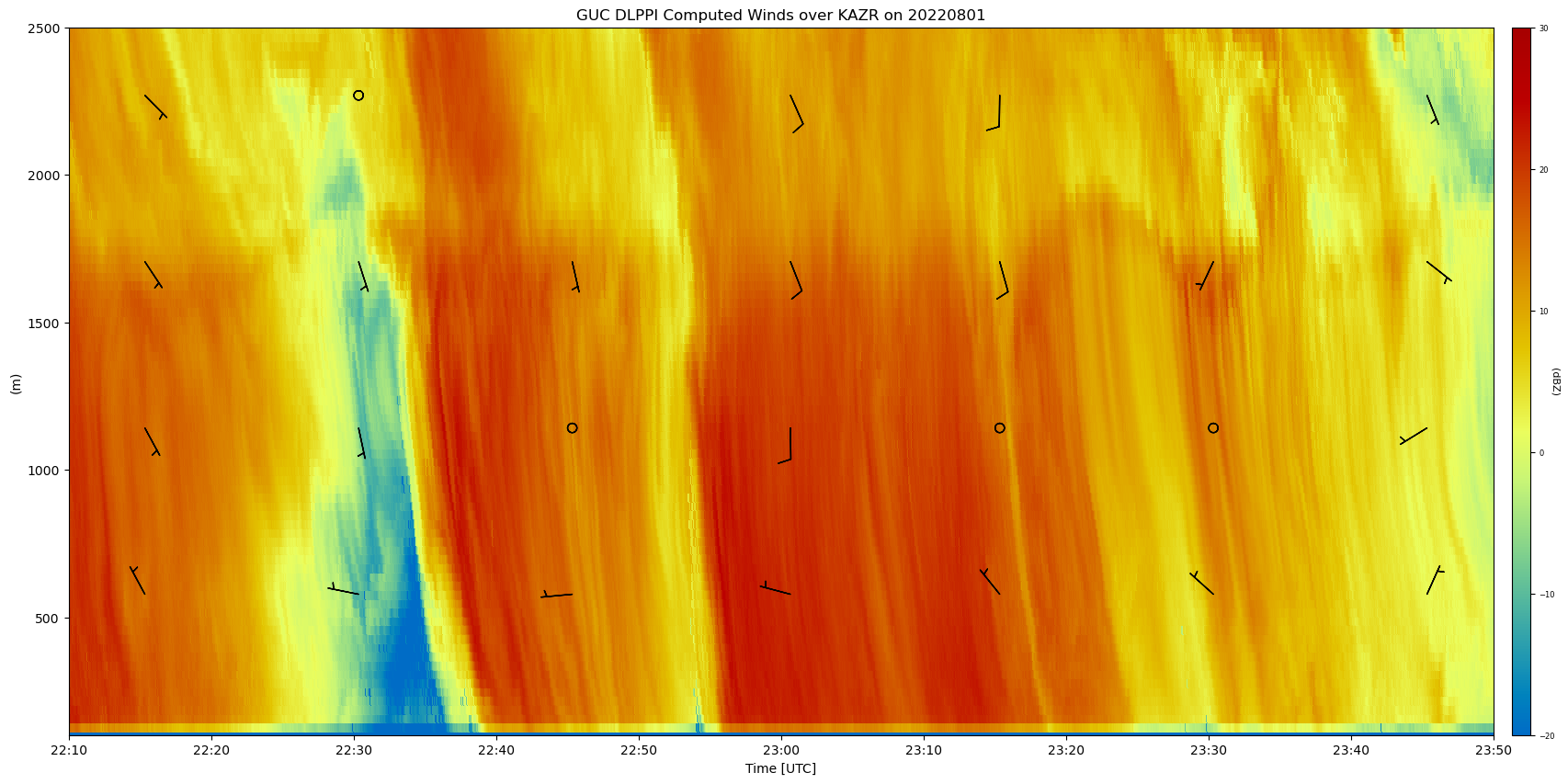
Add Doppler Lidar Retrieved Winds

# Specify datastream and date range for KAZR data
ds_dl = 'gucdlppiM1.b1'
startdate = '2022-08-01'
enddate = '2022-08-01'

# act.discovery.download_data(username, token, ds_dl, startdate, enddate)
dl_ppi_files = glob.glob(''.join(['./', ds_dl, '/*cdf']))

multi_ds = []
# Index last 9 files for the 22:00 and 23:00 timeframe and loop through.
for file in sorted(dl_ppi_files[-9:]):
    ds = act.io.arm.read_arm_netcdf(file)
    # Calculate the winds for each gucdlppi dataset.
    wind_ds = act.retrievals.compute_winds_from_ppi(
        ds, remove_all_missing=True, snr_threshold=0.008
    )
    multi_ds.append(wind_ds)

wind_ds = xr.merge(multi_ds)

# Create a display object.
display = act.plotting.TimeSeriesDisplay(
    {
        "GUC DLPPI Computed Winds over KAZR": wind_ds,
        "guckazrcfrgeM1.a1": kazr_ds,
    },
    figsize=(20, 10),
)

# Plot the wind barbs overlayed on the KAZR reflectivity
display.plot(
    'reflectivity', dsname='guckazrcfrgeM1.a1', cmap='act_HomeyerRainbow', vmin=-20, vmax=30
)
display.plot_barbs_from_spd_dir(
    'wind_speed', 'wind_direction', dsname='GUC DLPPI Computed Winds over KAZR', invert_y_axis=False
)

# Update the x-limits to make sure both wind profiles are shown
# Update the y-limits to show plotted winds
display.axes[0].set_xlim([np.datetime64('2022-08-01T22:10'), np.datetime64('2022-08-01T23:50')])
display.axes[0].set_ylim([kazr.range.min(), 2500])
plt.show()

Conclusion

By comparing these datasets, we can see similar and differences between the two datasets, but overall the structure is comparable. We can see the usefulness of ACT to not only read ARM datasets, but datasets outside of ARM. These workflows allow for scientists to have many different tools to use different datasets for their research, as well as quality control checks which increases the confidence in the quality and calibration of the instrumentation.

New Docs   Exploration of data from the 2024 eclipse at SGP