Blending Observations from TRACER using Py-ART

The TRacking Aerosol Convection Interactions (TRACER) field experiment was a U.S. Department of Energy IOP with the goal of studying the lifecycle of convection over Houston as well as potential aerosol impacts on this lifecycle. Houston is uniquely suited for this kind of field experiment where seabreeze convection forms off of the coast of Houston in cleaner air conditions and then approaches the more polluted Houston region. For more information about the TRACER field experiment, click here.

This post will show how to plot overlays of Texas A&M University Lightning Mapping Array data over GOES and ARM CSAPR2 data for a case of wildfire smoke entraining into developing convection sampled during July 12 and 13, 2022. In addition, we highlight a case that was tracked by CSAPR2 for 90 minutes on June 17, 2022.

Imports

import pyart
import act
import matplotlib.pyplot as plt
import xarray as xr
import numpy as np
import s3fs
import cartopy.crs as ccrs
import pandas as pd

from scipy.spatial import KDTree

%matplotlib inline

GOES data access

All of the NOAA GOES satellite data are available on Amazon Web Services for download. Therefore, you can use the s3fs tool to download the required data. We will download band 13, which is the longwave infrared band of GOES. In order to only download the band 13 files, we will ensure that there is a “C13” in the filename as this denotes the band number for each file.

# Use the anonymous credentials to access public data
fs = s3fs.S3FileSystem(anon=True)

day_no = 168  # Day number of year (here is June 17th, 16th on leap year)
year = 2022
hour = 20
files = np.array(fs.ls("noaa-goes16/ABI-L1b-RadC/%d/%d/%02d/" % (year, day_no, hour)))
band = "13"
for fi in files:
    if "C13" in fi:
        print("Downloading %s" % fi)
        fs.get(fi, "../data/" + fi.split("/")[-1])

Downloading noaa-goes16/ABI-L1b-RadC/2022/168/20/OR_ABI-L1b-RadC-M6C13_G16_s20221682001178_e20221682003562_c20221682004026.nc
Downloading noaa-goes16/ABI-L1b-RadC/2022/168/20/OR_ABI-L1b-RadC-M6C13_G16_s20221682006178_e20221682008562_c20221682009028.nc
Downloading noaa-goes16/ABI-L1b-RadC/2022/168/20/OR_ABI-L1b-RadC-M6C13_G16_s20221682011178_e20221682013562_c20221682014023.nc
Downloading noaa-goes16/ABI-L1b-RadC/2022/168/20/OR_ABI-L1b-RadC-M6C13_G16_s20221682016178_e20221682018562_c20221682019019.nc
Downloading noaa-goes16/ABI-L1b-RadC/2022/168/20/OR_ABI-L1b-RadC-M6C13_G16_s20221682021178_e20221682023563_c20221682024031.nc
Downloading noaa-goes16/ABI-L1b-RadC/2022/168/20/OR_ABI-L1b-RadC-M6C13_G16_s20221682026178_e20221682028562_c20221682029025.nc
Downloading noaa-goes16/ABI-L1b-RadC/2022/168/20/OR_ABI-L1b-RadC-M6C13_G16_s20221682031178_e20221682033562_c20221682034018.nc
Downloading noaa-goes16/ABI-L1b-RadC/2022/168/20/OR_ABI-L1b-RadC-M6C13_G16_s20221682036178_e20221682038562_c20221682039022.nc
Downloading noaa-goes16/ABI-L1b-RadC/2022/168/20/OR_ABI-L1b-RadC-M6C13_G16_s20221682041178_e20221682043562_c20221682044024.nc
Downloading noaa-goes16/ABI-L1b-RadC/2022/168/20/OR_ABI-L1b-RadC-M6C13_G16_s20221682046178_e20221682048562_c20221682049023.nc
Downloading noaa-goes16/ABI-L1b-RadC/2022/168/20/OR_ABI-L1b-RadC-M6C13_G16_s20221682051178_e20221682053562_c20221682054018.nc
Downloading noaa-goes16/ABI-L1b-RadC/2022/168/20/OR_ABI-L1b-RadC-M6C13_G16_s20221682056178_e20221682058562_c20221682059029.nc

goes_ds = xr.open_dataset(
    "../data/OR_ABI-L1b-RadC-M6C13_G16_s20221932006173_e20221932008557_c20221932009023.nc"
)
goes_ds

<xarray.Dataset>
Dimensions:                                           (y: 1500, x: 2500,
                                                       number_of_time_bounds: 2,
                                                       number_of_image_bounds: 2,
                                                       band: 1,
                                                       num_star_looks: 24)
Coordinates:
    t                                                 datetime64[ns] 2022-07-...
  * y                                                 (y) float64 0.1282 ... ...
  * x                                                 (x) float64 -0.1013 ......
    y_image                                           float32 0.08624
    x_image                                           float32 -0.03136
    band_id                                           (band) int8 13
    band_wavelength                                   (band) float32 10.33
    t_star_look                                       (num_star_looks) datetime64[ns] ...
    band_wavelength_star_look                         (num_star_looks) float32 ...
Dimensions without coordinates: number_of_time_bounds, number_of_image_bounds,
                                band, num_star_looks
Data variables: (12/37)
    Rad                                               (y, x) float32 ...
    DQF                                               (y, x) float32 ...
    time_bounds                                       (number_of_time_bounds) datetime64[ns] ...
    goes_imager_projection                            int32 -2147483647
    y_image_bounds                                    (number_of_image_bounds) float32 ...
    x_image_bounds                                    (number_of_image_bounds) float32 ...
    ...                                                ...
    algorithm_dynamic_input_data_container            int32 -2147483647
    processing_parm_version_container                 int32 -2147483647
    algorithm_product_version_container               int32 -2147483647
    star_id                                           (num_star_looks) float32 ...
    channel_integration_time                          float64 336.0
    channel_gain_field                                float64 0.0
Attributes: (12/30)
    naming_authority:          gov.nesdis.noaa
    Conventions:               CF-1.7
    standard_name_vocabulary:  CF Standard Name Table (v35, 20 July 2016)
    institution:               DOC/NOAA/NESDIS > U.S. Department of Commerce,...
    project:                   GOES
    production_site:           WCDAS
    ...                        ...
    timeline_id:               ABI Mode 6
    date_created:              2022-07-12T20:09:02.3Z
    time_coverage_start:       2022-07-12T20:06:17.3Z
    time_coverage_end:         2022-07-12T20:08:55.7Z
    LUT_Filenames:             SpaceLookParams(FM1A_CDRL79RevP_PR_09_00_02)-6...
    id:                        f45b564c-dcb9-498a-ac56-da80a1d735a5

xarray.Dataset

• Dimensions:
  • y: 1500
  • x: 2500
  • number_of_time_bounds: 2
  • number_of_image_bounds: 2
  • band: 1
  • num_star_looks: 24
• Coordinates: (9)
  • t
    ()
    datetime64[ns]
    ...

    long_name :

    J2000 epoch mid-point between the start and end image scan in seconds

    standard_name :

    time

    axis :

    T

    bounds :

    time_bounds

    array('2022-07-12T20:07:36.537394048', dtype='datetime64[ns]')

  • y
    (y)
    float64
    0.1282 0.1282 ... 0.04432 0.04427

    units :

    rad

    axis :

    Y

    long_name :

    GOES fixed grid projection y-coordinate

    standard_name :

    projection_y_coordinate

    array([0.128212, 0.128156, 0.1281  , ..., 0.04438 , 0.044324, 0.044268])

  • x
    (x)
    float64
    -0.1013 -0.1013 ... 0.03856 0.03861

    units :

    rad

    axis :

    X

    long_name :

    GOES fixed grid projection x-coordinate

    standard_name :

    projection_x_coordinate

    array([-0.101332, -0.101276, -0.10122 , ...,  0.0385  ,  0.038556,  0.038612])

  • y_image
    ()
    float32
    ...

    long_name :

    GOES-R fixed grid projection y-coordinate center of image

    standard_name :

    projection_y_coordinate

    units :

    rad

    axis :

    Y

    array(0.08624, dtype=float32)

  • x_image
    ()
    float32
    ...

    long_name :

    GOES-R fixed grid projection x-coordinate center of image

    standard_name :

    projection_x_coordinate

    units :

    rad

    axis :

    X

    array(-0.03136, dtype=float32)

  • band_id
    (band)
    int8
    ...

    long_name :

    ABI band number

    standard_name :

    sensor_band_identifier

    units :

    1

    array([13], dtype=int8)

  • band_wavelength
    (band)
    float32
    ...

    long_name :

    ABI band central wavelength

    standard_name :

    sensor_band_central_radiation_wavelength

    units :

    um

    array([10.33], dtype=float32)

  • t_star_look
    (num_star_looks)
    datetime64[ns]
    ...

    long_name :

    J2000 epoch time of star observed in seconds

    standard_name :

    time

    axis :

    T

    array(['2000-01-01T11:43:21.000000000', '2000-01-01T11:43:21.000000000',
           '2000-01-01T11:43:21.000000000', '2000-01-01T11:43:21.000000000',
           '2000-01-01T11:43:21.000000000', '2000-01-01T11:43:21.000000000',
           '2000-01-01T11:43:21.000000000', '2000-01-01T11:43:21.000000000',
           '2000-01-01T11:43:21.000000000', '2000-01-01T11:43:21.000000000',
           '2000-01-01T11:43:21.000000000', '2000-01-01T11:43:21.000000000',
           '2000-01-01T11:43:21.000000000', '2000-01-01T11:43:21.000000000',
           '2000-01-01T11:43:21.000000000', '2000-01-01T11:43:21.000000000',
           '2000-01-01T11:43:21.000000000', '2000-01-01T11:43:21.000000000',
           '2000-01-01T11:43:21.000000000', '2000-01-01T11:43:21.000000000',
           '2000-01-01T11:43:21.000000000', '2000-01-01T11:43:21.000000000',
           '2000-01-01T11:43:21.000000000', '2000-01-01T11:43:21.000000000'],
          dtype='datetime64[ns]')

  • band_wavelength_star_look
    (num_star_looks)
    float32
    ...

    long_name :

    ABI band central wavelength associated with observed star

    standard_name :

    sensor_band_central_radiation_wavelength

    units :

    um

    array([-999., -999., -999., -999., -999., -999., -999., -999., -999., -999.,
           -999., -999., -999., -999., -999., -999., -999., -999., -999., -999.,
           -999., -999., -999., -999.], dtype=float32)

• Data variables: (37)
  • Rad
    (y, x)
    float32
    ...

    long_name :

    ABI L1b Radiances

    standard_name :

    toa_outgoing_radiance_per_unit_wavenumber

    sensor_band_bit_depth :

    12

    valid_range :

    [ 0 4094]

    units :

    mW m-2 sr-1 (cm-1)-1

    resolution :

    y: 0.000056 rad x: 0.000056 rad

    grid_mapping :

    goes_imager_projection

    cell_methods :

    t: point area: point

    ancillary_variables :

    DQF

    [3750000 values with dtype=float32]

  • DQF
    (y, x)
    float32
    ...

    long_name :

    ABI L1b Radiances data quality flags

    standard_name :

    status_flag

    valid_range :

    [0 4]

    units :

    1

    grid_mapping :

    goes_imager_projection

    cell_methods :

    t: point area: point

    flag_values :

    [0 1 2 3 4]

    flag_meanings :

    good_pixel_qf conditionally_usable_pixel_qf out_of_range_pixel_qf no_value_pixel_qf focal_plane_temperature_threshold_exceeded_qf

    number_of_qf_values :

    5

    percent_good_pixel_qf :

    1.0

    percent_conditionally_usable_pixel_qf :

    0.0

    percent_out_of_range_pixel_qf :

    0.0

    percent_no_value_pixel_qf :

    0.0

    percent_focal_plane_temperature_threshold_exceeded_qf :

    0.0

    [3750000 values with dtype=float32]

  • time_bounds
    (number_of_time_bounds)
    datetime64[ns]
    ...

    long_name :

    Scan start and end times in seconds since epoch (2000-01-01 12:00:00)

    array(['2022-07-12T20:06:17.326423040', '2022-07-12T20:08:55.748365056'],
          dtype='datetime64[ns]')

  • goes_imager_projection
    ()
    int32
    ...

    long_name :

    GOES-R ABI fixed grid projection

    grid_mapping_name :

    geostationary

    perspective_point_height :

    35786023.0

    semi_major_axis :

    6378137.0

    semi_minor_axis :

    6356752.31414

    inverse_flattening :

    298.2572221

    latitude_of_projection_origin :

    0.0

    longitude_of_projection_origin :

    -75.0

    sweep_angle_axis :

    x

    array(-2147483647, dtype=int32)

  • y_image_bounds
    (number_of_image_bounds)
    float32
    ...

    long_name :

    GOES-R fixed grid projection y-coordinate north/south extent of image

    units :

    rad

    array([0.12824, 0.04424], dtype=float32)

  • x_image_bounds
    (number_of_image_bounds)
    float32
    ...

    long_name :

    GOES-R fixed grid projection x-coordinate west/east extent of image

    units :

    rad

    array([-0.10136,  0.03864], dtype=float32)

  • nominal_satellite_subpoint_lat
    ()
    float32
    ...

    long_name :

    nominal satellite subpoint latitude (platform latitude)

    standard_name :

    latitude

    units :

    degrees_north

    array(0.)

  • nominal_satellite_subpoint_lon
    ()
    float32
    ...

    long_name :

    nominal satellite subpoint longitude (platform longitude)

    standard_name :

    longitude

    units :

    degrees_east

    array(-75.199997)

  • nominal_satellite_height
    ()
    float32
    ...

    long_name :

    nominal satellite height above GRS 80 ellipsoid (platform altitude)

    standard_name :

    height_above_reference_ellipsoid

    units :

    km

    array(35786.023438)

  • geospatial_lat_lon_extent
    ()
    float32
    ...

    long_name :

    geospatial latitude and longitude references

    geospatial_westbound_longitude :

    -152.10928

    geospatial_northbound_latitude :

    56.76145

    geospatial_eastbound_longitude :

    -52.94688

    geospatial_southbound_latitude :

    14.57134

    geospatial_lat_center :

    30.083002

    geospatial_lon_center :

    -87.096954

    geospatial_lat_nadir :

    0.0

    geospatial_lon_nadir :

    -75.0

    geospatial_lat_units :

    degrees_north

    geospatial_lon_units :

    degrees_east

    array(9.96921e+36, dtype=float32)

  • yaw_flip_flag
    ()
    float32
    ...

    long_name :

    Flag indicating the spacecraft is operating in yaw flip configuration

    valid_range :

    [0 1]

    units :

    1

    flag_values :

    [0 1]

    flag_meanings :

    false true

    array(0.)

  • esun
    ()
    float32
    ...

    long_name :

    bandpass-weighted solar irradiance at the mean Earth-Sun distance

    standard_name :

    toa_shortwave_irradiance_per_unit_wavelength

    units :

    W m-2 um-1

    cell_methods :

    t: mean

    array(nan)

  • kappa0
    ()
    float32
    ...

    long_name :

    Inverse of the incoming top of atmosphere radiance at current earth-sun distance (PI d2 esun-1)-1, where d is the ratio of instantaneous Earth-Sun distance divided by the mean Earth-Sun distance, esun is the bandpass-weighted solar irradiance and PI is a standard constant used to convert ABI L1b radiance to reflectance

    units :

    (W m-2 um-1)-1

    cell_methods :

    t: mean

    array(nan)

  • planck_fk1
    ()
    float32
    ...

    long_name :

    wavenumber-dependent coefficient (2 h c2/ nu3) used in the ABI emissive band monochromatic brightness temperature computation, where nu =central wavenumber and h and c are standard constants

    units :

    W m-1

    array(10803.299805)

  • planck_fk2
    ()
    float32
    ...

    long_name :

    wavenumber-dependent coefficient (h c nu/b) used in the ABI emissive band monochromatic brightness temperature computation, where nu = central wavenumber and h, c, and b are standard constants

    units :

    K

    array(1392.73999)

  • planck_bc1
    ()
    float32
    ...

    long_name :

    spectral bandpass correction offset for brightness temperature (B(nu) - bc_1)/bc_2 where B()=planck_function() and nu=wavenumber

    units :

    K

    array(0.0755)

  • planck_bc2
    ()
    float32
    ...

    long_name :

    spectral bandpass correction scale factor for brightness temperature (B(nu) - bc_1)/bc_2 where B()=planck_function() and nu=wavenumber

    units :

    1

    array(0.99975)

  • valid_pixel_count
    ()
    float64
    ...

    long_name :

    number of good and conditionally usable pixels

    units :

    count

    grid_mapping :

    goes_imager_projection

    cell_methods :

    t: sum area: sum (interval: 0.000056 rad comment: good and conditionally usable quality pixels only)

    array(3702838.)

  • missing_pixel_count
    ()
    float64
    ...

    long_name :

    number of missing pixels

    units :

    count

    grid_mapping :

    goes_imager_projection

    cell_methods :

    t: sum area: sum (interval: 0.000056 rad comment: missing ABI fixed grid pixels only)

    array(0.)

  • saturated_pixel_count
    ()
    float64
    ...

    long_name :

    number of saturated pixels

    units :

    count

    grid_mapping :

    goes_imager_projection

    cell_methods :

    t: sum area: sum (interval: 0.000056 rad comment: radiometrically saturated geolocated/not missing pixels only)

    array(0.)

  • undersaturated_pixel_count
    ()
    float64
    ...

    long_name :

    number of undersaturated pixels

    units :

    count

    grid_mapping :

    goes_imager_projection

    cell_methods :

    t: sum area: sum (interval: 0.000056 rad comment: radiometrically undersaturated geolocated/not missing pixels only)

    array(0.)

  • focal_plane_temperature_threshold_exceeded_count
    ()
    float64
    ...

    long_name :

    number of pixels whose temperatures exceeded the threshold

    units :

    count

    grid_mapping :

    goes_imager_projection

    cell_methods :

    t: sum area: sum (interval: 0.000056 rad comment: temperature exceeded pixels only)

    array(0.)

  • min_radiance_value_of_valid_pixels
    ()
    float32
    ...

    long_name :

    minimum radiance value of pixels

    standard_name :

    toa_outgoing_radiance_per_unit_wavenumber

    valid_range :

    [ -1.6443 185.5699]

    units :

    mW m-2 sr-1 (cm-1)-1

    grid_mapping :

    goes_imager_projection

    cell_methods :

    t: sum area: minimum (interval: 0.000056 rad comment: good and conditionally usable quality pixels only)

    array(8.849287)

  • max_radiance_value_of_valid_pixels
    ()
    float32
    ...

    long_name :

    maximum radiance value of pixels

    standard_name :

    toa_outgoing_radiance_per_unit_wavenumber

    valid_range :

    [ -1.6443 185.5699]

    units :

    mW m-2 sr-1 (cm-1)-1

    grid_mapping :

    goes_imager_projection

    cell_methods :

    t: sum area: maximum (interval: 0.000056 rad comment: good and conditionally usable quality pixels only)

    array(154.23053)

  • mean_radiance_value_of_valid_pixels
    ()
    float32
    ...

    long_name :

    mean radiance value of pixels

    standard_name :

    toa_outgoing_radiance_per_unit_wavenumber

    valid_range :

    [ -1.6443 185.5699]

    units :

    mW m-2 sr-1 (cm-1)-1

    grid_mapping :

    goes_imager_projection

    cell_methods :

    t: sum area: mean (interval: 0.000056 rad comment: good and conditionally usable quality pixels only)

    array(85.197975)

  • std_dev_radiance_value_of_valid_pixels
    ()
    float32
    ...

    long_name :

    standard deviation of radiance values of pixels

    standard_name :

    toa_outgoing_radiance_per_unit_wavenumber

    units :

    mW m-2 sr-1 (cm-1)-1

    grid_mapping :

    goes_imager_projection

    cell_methods :

    t: sum area: standard_deviation (interval: 0.000056 rad comment: good and conditionally usable quality pixels only)

    array(24.985853)

  • maximum_focal_plane_temperature
    ()
    float32
    ...

    long_name :

    maximum focal plane temperature value

    valid_range :

    [ 0. 999.]

    units :

    K

    array(59.951939)

  • focal_plane_temperature_threshold_increasing
    ()
    float32
    ...

    long_name :

    focal plane temperature threshold increasing bounds value

    valid_range :

    [ 0. 999.]

    units :

    K

    array(81.)

  • focal_plane_temperature_threshold_decreasing
    ()
    float32
    ...

    long_name :

    focal plane temperature threshold decreasing bounds value

    valid_range :

    [ 0. 999.]

    units :

    K

    array(81.)

  • percent_uncorrectable_L0_errors
    ()
    float32
    ...

    long_name :

    percent data lost due to uncorrectable L0 errors

    valid_range :

    [0. 1.]

    units :

    percent

    grid_mapping :

    goes_imager_projection

    cell_methods :

    t: sum area: sum (uncorrectable L0 errors only)

    array(0.)

  • earth_sun_distance_anomaly_in_AU
    ()
    float32
    ...

    long_name :

    earth sun distance anomaly in astronomical units

    units :

    ua

    cell_methods :

    t: mean

    array(1.016543)

  • algorithm_dynamic_input_data_container
    ()
    int32
    ...

    long_name :

    container for filenames of dynamic algorithm input data

    input_ABI_L0_data :

    OR_ABI-L0-C-M6_G16_s20221932006173_e20221932008557_c*.nc

    array(-2147483647, dtype=int32)

  • processing_parm_version_container
    ()
    int32
    ...

    long_name :

    container for processing parameter filenames

    L1b_processing_parm_version :

    OR-PARM-RAD_G16_v01r00.zip

    array(-2147483647, dtype=int32)

  • algorithm_product_version_container
    ()
    int32
    ...

    long_name :

    container for algorithm package filename and product version

    algorithm_version :

    OR_ABI-L1b-ALG-RAD_v01r00.zip

    product_version :

    v01r00

    array(-2147483647, dtype=int32)

  • star_id
    (num_star_looks)
    float32
    ...

    long_name :

    ABI star catalog identifier associated with observed star

    array([nan, nan, nan, nan, nan, nan, nan, nan, nan, nan, nan, nan, nan, nan,
           nan, nan, nan, nan, nan, nan, nan, nan, nan, nan], dtype=float32)

  • channel_integration_time
    ()
    float64
    ...

    long_name :

    Channel-dependent Channel Integration Time, as defined in the VNIR or IR Channel Configuration Table Telemetry

    units :

    count

    array(336.)

  • channel_gain_field
    ()
    float64
    ...

    long_name :

    Channel-dependent Gain Field, as defined in the VNIR or IR Channel Configuration Table Telemetry

    units :

    1

    array(0.)

• Attributes: (30)

  naming_authority :

  gov.nesdis.noaa

  Conventions :

  CF-1.7

  standard_name_vocabulary :

  CF Standard Name Table (v35, 20 July 2016)

  institution :

  DOC/NOAA/NESDIS > U.S. Department of Commerce, National Oceanic and Atmospheric Administration, National Environmental Satellite, Data, and Information Services

  project :

  GOES

  production_site :

  WCDAS

  production_environment :

  OE

  spatial_resolution :

  2km at nadir

  Metadata_Conventions :

  Unidata Dataset Discovery v1.0

  orbital_slot :

  GOES-East

  platform_ID :

  G16

  instrument_type :

  GOES-R Series Advanced Baseline Imager (ABI)

  scene_id :

  CONUS

  instrument_ID :

  FM1

  title :

  ABI L1b Radiances

  summary :

  Single emissive band ABI L1b Radiance Products are digital maps of outgoing radiance values at the top of the atmosphere for IR bands.

  keywords :

  SPECTRAL/ENGINEERING > INFRARED WAVELENGTHS > INFRARED RADIANCE

  keywords_vocabulary :

  NASA Global Change Master Directory (GCMD) Earth Science Keywords, Version 7.0.0.0.0

  iso_series_metadata_id :

  a70be540-c38b-11e0-962b-0800200c9a66

  license :

  Unclassified data. Access is restricted to approved users only.

  processing_level :

  National Aeronautics and Space Administration (NASA) L1b

  cdm_data_type :

  Image

  dataset_name :

  OR_ABI-L1b-RadC-M6C13_G16_s20221932006173_e20221932008557_c20221932009023.nc

  production_data_source :

  Realtime

  timeline_id :

  ABI Mode 6

  date_created :

  2022-07-12T20:09:02.3Z

  time_coverage_start :

  2022-07-12T20:06:17.3Z

  time_coverage_end :

  2022-07-12T20:08:55.7Z

  LUT_Filenames :

  SpaceLookParams(FM1A_CDRL79RevP_PR_09_00_02)-637827000.0.h5 QTableBand13(FM1A_CDRL79RevH_DO_08_00_00)-582860861.0.h5 CalTargetTimeIntervals(FM1A_CDRL79RevP_DO_08_00_01)-611906620.0.h5 BandSaturationLimits(FM1A_CDRL79RevH_DO_08_00_00)-600000000.0.h5 SolarSpaceLookParams(FM1A_ADR1233_PR_09_08_25)-709281036.0.h5 DeadRowListParams(FM1A_CDRL79RevH_DO_08_00_00)-600000000.0.h5 Mirror_Record(FM1A_CDRL79RevG_DO_07_00_00)-582860861.0.h5 KalmanAstroConsts(FM1A_CDRL79RevH_DO_08_00_00)-600000000.0.xml KalmanFilterControls(FM1A_PR_09_08_02)-677650371.0.xml KalmanMeasMaxSensibles(FMAA_INT_ONLY_DO_09_01_00)-652936814.0.xml KalmanPreprocessorControls(FM1A_CDRL79RevJ_PR_09_06_02)-657795700.0.xml KalmanReferenceData(FM1A_CDRL79RevH_DO_08_00_00)-888.0.xml KalmanStarCatalogs(FM1A_CDRL79RevH_DO_08_00_00)-600000000.0.xml ABI_NavigationRDP_Band13(FM1A_CDRL79RevJ_DO_07_00_00)-582860861.0.xml ABI_NavigationParameters_Band13(FM1A_CDRL79RevH_DO_07_00_00)-582860861.0.xml ABI_ResamplingImplementation_Band13(FM1A_CDRL79RevH_DO_07_02_00)-602129336.0.xml ABI_ResamplingParameters_Band13(FM1A_CDRL79RevJ_DO_07_00_00)-582860861.0.xml StarLookParams(FM1A_CDRL79RevH_DO_08_00_00)-600000000.0.h5 StarDetectionParams(FM1A_CDRL79RevJ_DO_07_00_00)-582860861.0.xml ResamplingScaledConversion(FMAA_INT_ONLY_DO_08_00_00)-1111.0.xml BlockReleaseRegions(FMAA_INT_ONLY_DO_08_00_00)-2222.0.csv IR_RetrievalParameters(FM1A_CDRL79RevH_DO_09_01_00)-652936750.0.h5 RadianceLUT_Band13(FM1A_CDRL79RevE_DO_08_00_00)-582860861.0.h5 ICT_Record(FM1A_TMABI_18_159_PR_09_00_02)-637827000.0.h5 ICM_ConversionConsts(FM1A_CDRL43-18_DO_09_01_00)-652936750.0.h5 ICM_SensorCoefficients(FM1A_TMABI_18_159_TMABI_18_533_DO_09_05_00)-676949608.0.h5

  id :

  f45b564c-dcb9-498a-ac56-da80a1d735a5

The following code in Python was created by the NOAA/NESDIS/STAR Aerosols and Atmospheric Composition Science Team to convert the GOES projection values to lat/lon coordinates that are more useful for selecting a sub-domain of GOES to plot. The original code used the netCDF4 library, so it was adapted to xarray by Bobby Jackson.

# Calculate latitude and longitude from GOES ABI fixed grid projection data
# GOES ABI fixed grid projection is a map projection relative to the GOES satellite
# Units: latitude in °N (°S < 0), longitude in °E (°W < 0)
# See GOES-R Product User Guide (PUG) Volume 5 (L2 products) Section 4.2.8 for details & example of calculations
# "file_id" is an ABI L1b or L2 .nc file opened using the netCDF4 library


def calculate_degrees(file_id):
    # Read in GOES ABI fixed grid projection variables and constants
    x_coordinate_1d = file_id.variables["x"][:]  # E/W scanning angle in radians
    y_coordinate_1d = file_id.variables["y"][:]  # N/S elevation angle in radians
    projection_info = file_id.variables["goes_imager_projection"]
    lon_origin = projection_info.attrs["longitude_of_projection_origin"]
    H = (
        projection_info.attrs["perspective_point_height"]
        + projection_info.attrs["semi_major_axis"]
    )
    r_eq = projection_info.attrs["semi_major_axis"]
    r_pol = projection_info.attrs["semi_minor_axis"]

    # Create 2D coordinate matrices from 1D coordinate vectors
    x_coordinate_2d, y_coordinate_2d = np.meshgrid(x_coordinate_1d, y_coordinate_1d)

    # Equations to calculate latitude and longitude
    lambda_0 = (lon_origin * np.pi) / 180.0
    a_var = np.power(np.sin(x_coordinate_2d), 2.0) + (
        np.power(np.cos(x_coordinate_2d), 2.0)
        * (
            np.power(np.cos(y_coordinate_2d), 2.0)
            + (
                ((r_eq * r_eq) / (r_pol * r_pol))
                * np.power(np.sin(y_coordinate_2d), 2.0)
            )
        )
    )
    b_var = -2.0 * H * np.cos(x_coordinate_2d) * np.cos(y_coordinate_2d)
    c_var = (H**2.0) - (r_eq**2.0)
    r_s = (-1.0 * b_var - np.sqrt((b_var**2) - (4.0 * a_var * c_var))) / (2.0 * a_var)
    s_x = r_s * np.cos(x_coordinate_2d) * np.cos(y_coordinate_2d)
    s_y = -r_s * np.sin(x_coordinate_2d)
    s_z = r_s * np.cos(x_coordinate_2d) * np.sin(y_coordinate_2d)

    # Ignore numpy errors for sqrt of negative number; occurs for GOES-16 ABI CONUS sector data
    np.seterr(all="ignore")

    abi_lat = (180.0 / np.pi) * (
        np.arctan(
            ((r_eq * r_eq) / (r_pol * r_pol))
            * ((s_z / np.sqrt(((H - s_x) * (H - s_x)) + (s_y * s_y))))
        )
    )
    abi_lon = (lambda_0 - np.arctan(s_y / (H - s_x))) * (180.0 / np.pi)

    return abi_lat, abi_lon

Calculate the latitude and longitude coordinates of the GOES data and then crop the data to our region of interest: 25 to 35 \(^{\circ} N\) and 100 to 95 \(^{\circ} W\).

lat, lon = calculate_degrees(goes_ds)
lat = np.nan_to_num(lat, -9999)
lon = np.nan_to_num(lon, -9999)
lat_range = (25.0, 35.0)
lon_range = (-100.0, -95.0)
lat_min = lat.min(axis=1)
lat_max = lat.max(axis=1)
lat_min_bound = np.argmin(np.abs(lat_min - lat_range[0]))
lat_max_bound = np.argmin(np.abs(lat_max - lat_range[1]))
lon_min = lon.min(axis=0)
lon_max = lon.max(axis=0)
lon_min_bound = np.argmin(np.abs(lon_min - lon_range[0]))
lon_max_bound = np.argmin(np.abs(lon_max - lon_range[1]))

CSAPR data access

The a1-level CSAPR data are available for public use on ARM Data Disovery. In addition, we can use the Atmospheric Community Toolkit to download the July 12 and 13 CSAPR data. The DOI for the CSAPR2 a1-level data is 10.5439/1467901, which if accessed will bring you to the download page on ARM Data Discovery.

The first block of code below will look at the automated catalogue of CSAPR data created by Adam Theisen. This provides us with a view of what scanning mode the CSAPR was in for a given time period as well as the scanning geometry and precipitation coverage.

cell_track_info = pd.read_csv(
    "https://raw.githubusercontent.com/AdamTheisen/cell-track-stats/main/data/houcsapr.20220617.csv",
    index_col=["time"],
    parse_dates=True,
)
cell_track_info

	Unnamed: 0	scan_mode	scan_name	template_name	azimuth_min	azimuth_max	elevation_min	elevation_max	range_min	range_max	cell_azimuth	cell_range	cell_zh	ngates_gt_0	ngates_gt_10	ngates_gt_30	ngates_gt_50	ngates_gt_10_5km	ngates_gt40_5km	ngates
time
2022-06-17 00:00:03	0	rhi	rhi	hou-rhi-cell-track-05-deg	303.74450	303.74450	0.637207	4.383545	0.0	109900.0	NaN	NaN	NaN	0	0	0	0	0	0	0
2022-06-17 00:06:09	1	ppi	ppi	hou-ppi-cell-track-05-deg	297.59216	307.63367	3.021240	3.988037	0.0	109900.0	297.910767	700.0	30.930866	59	30	3	0	0	0	78
2022-06-17 00:06:40	2	rhi	rhi	hou-rhi-cell-track-05-deg	302.64587	302.64587	0.637207	4.383545	0.0	109900.0	302.645874	1800.0	-0.776333	0	0	0	0	0	0	2
2022-06-17 00:06:59	3	rhi	rhi	hou-rhi-cell-track-05-deg	302.55798	302.59094	0.637207	4.383545	0.0	109900.0	NaN	NaN	NaN	0	0	0	0	0	0	0
2022-06-17 00:07:18	4	rhi	rhi	hou-rhi-cell-track-05-deg	302.97546	302.99744	0.637207	4.383545	0.0	109900.0	302.975464	900.0	-2.972101	0	0	0	0	0	0	2
...	...	...	...	...	...	...	...	...	...	...	...	...	...	...	...	...	...	...	...	...
2022-06-17 23:39:46	2826	rhi	rhi	hou-rhi-cell-track-10-deg	301.48132	301.50330	0.648193	9.382324	0.0	109900.0	301.503296	62400.0	40.327583	990	989	210	0	134	0	995
2022-06-17 23:40:02	2827	rhi	rhi	hou-rhi-cell-track-10-deg	305.70007	305.70007	0.648193	9.404297	0.0	109900.0	305.700073	13600.0	29.037998	12	6	0	0	0	0	20
2022-06-17 23:40:16	2828	rhi	rhi	hou-rhi-cell-track-10-deg	297.23510	297.26807	0.648193	9.382324	0.0	109900.0	297.235107	700.0	28.459156	28	25	0	0	0	0	34
2022-06-17 23:40:29	2829	ppi	ppi	hou-ppi-cell-track-10-deg	296.08704	306.16150	2.999268	6.998291	0.0	109900.0	300.646362	59100.0	33.882927	807	783	27	0	63	0	830
2022-06-17 23:40:54	2830	rhi	rhi	hou-rhi-cell-track-10-deg	301.05835	301.08032	0.648193	9.382324	0.0	109900.0	301.058350	62800.0	37.198204	767	767	75	0	76	0	773

2831 rows × 20 columns

For this notebook we are interested in the time periods where the CSAPR was scanning in PPI mode. For this entire time period, the CSAPR was in cell-tracking mode, meaning that it was focused on a single convective cell in the Houston region. This scanning strategy will have a much more frequent scans over a smaller area covered by a single convective cell and is designed to track the lifecycle of a convective cell.

start_hour = 20
end_hour = 21
print("All PPI scan times between %d UTC and %d UTC:" % (start_hour, end_hour))
for index in cell_track_info.index:
    if index.hour >= 20 and index.hour < end_hour:
        if cell_track_info.loc[index].scan_mode == "ppi":
            print(index)

All PPI scan times between 20 UTC and 21 UTC:
2022-06-17 20:00:07
2022-06-17 20:00:51
2022-06-17 20:01:34
2022-06-17 20:02:17
2022-06-17 20:03:05
2022-06-17 20:03:48
2022-06-17 20:04:31
2022-06-17 20:05:22
2022-06-17 20:06:08
2022-06-17 20:06:59
2022-06-17 20:07:43
2022-06-17 20:08:29
2022-06-17 20:09:15
2022-06-17 20:09:56
2022-06-17 20:10:53
2022-06-17 20:11:39
2022-06-17 20:14:24
2022-06-17 20:16:25
2022-06-17 20:18:27
2022-06-17 20:20:25
2022-06-17 20:22:31
2022-06-17 20:24:30
2022-06-17 20:26:31
2022-06-17 20:28:30
2022-06-17 20:30:31
2022-06-17 20:32:29
2022-06-17 20:34:30
2022-06-17 20:36:30
2022-06-17 20:38:31
2022-06-17 20:40:32
2022-06-17 20:42:33
2022-06-17 20:44:31
2022-06-17 20:46:31
2022-06-17 20:48:25
2022-06-17 20:50:27
2022-06-17 20:52:21
2022-06-17 20:54:20
2022-06-17 20:56:22
2022-06-17 20:57:51
2022-06-17 20:59:19

csapr = pyart.io.read(
    "/Users/rjackson/TRACER-PAWS-NEXRAD-LMA/data/houcsapr2cfrS2.a1.20220712.200714.nc"
)

Load LMA Flash data

Here we load the data from the Houston Lightning Mapping Array. The data are in standard netCDF format that is easily read by xarray. The data are currently available for order at https://data.eol.ucar.edu/cgi-bin/codiac/fgr_form/id=100.016. Both the flash density data and locations of each flash are stored in the file.

lma_ds = xr.open_dataset(
    "/Users/rjackson/TRACER-PAWS-NEXRAD-LMA/data/LYLOUT_220712_000000_86400_map500m.nc"
)

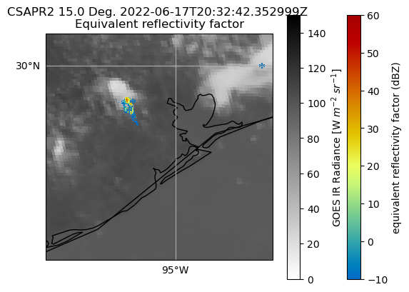
June 17th case

This is a case of a storm that was tracked by CSAPR for about 90 minutes during the afternoon of June 17th 2022. We will use the same code from above to plot the radar/LMA overlays over the GOES IR radiance data for this case. This first block of code combines the above code to load and subset all of the necessary data for the overlays.

goes_ds = xr.open_dataset(
    "../data/OR_ABI-L1b-RadC-M6C13_G16_s20221682056178_e20221682058562_c20221682059029.nc"
)
csapr = pyart.io.read(
    "/Users/rjackson/TRACER-PAWS-NEXRAD-LMA/data/houcsapr2cfrS2.a1.20220617.203229.nc"
)
lma_ds = xr.open_dataset(
    "/Users/rjackson/TRACER-PAWS-NEXRAD-LMA/data/LYLOUT_220617_000000_86400_map500m.nc"
)
lma_ds
lat, lon = calculate_degrees(goes_ds)
lat = np.nan_to_num(lat, -9999)
lon = np.nan_to_num(lon, -9999)
lat_range = (25.0, 35.0)
lon_range = (-100.0, -95.0)
lat_min = lat.min(axis=1)
lat_max = lat.max(axis=1)
lat_min_bound = np.argmin(np.abs(lat_min - lat_range[0]))
lat_max_bound = np.argmin(np.abs(lat_max - lat_range[1]))
lon_min = lon.min(axis=0)
lon_max = lon.max(axis=0)
lon_min_bound = np.argmin(np.abs(lon_min - lon_range[0]))
lon_max_bound = np.argmin(np.abs(lon_max - lon_range[1]))

Here, we use cartopy to plot the GOES/LMA data and then the RadarMapDisplay object to overlay the radar data on top of the GOES/LMA data.

fig, ax = plt.subplots(1, 1, subplot_kw=dict(projection=ccrs.PlateCarree()))
Rad = goes_ds.Rad.values[lat_max_bound:lat_min_bound, lon_max_bound:lon_min_bound]
gatefilter = pyart.filters.GateFilter(csapr)
gatefilter.exclude_below("normalized_coherent_power", 0.50)

disp = pyart.graph.RadarMapDisplay(csapr)
c = ax.pcolormesh(
    lon[lat_max_bound:lat_min_bound, lon_max_bound:lon_min_bound],
    lat[lat_max_bound:lat_min_bound, lon_max_bound:lon_min_bound],
    Rad,
    cmap="binary",
    vmin=0,
    vmax=150,
)
disp.plot_ppi_map(
    "reflectivity", gatefilter=gatefilter, ax=ax, sweep=1, vmin=-10, vmax=60
)

plt.colorbar(c, label="GOES IR Radiance [W $m^{-2}\ sr^{-1}]$")

flash_times = np.squeeze(
    np.argwhere(
        np.logical_and(
            lma_ds.flash_time_start.values > np.datetime64("2022-06-17T20:31:00"),
            lma_ds.flash_time_start.values < np.datetime64("2022-06-17T20:33:00"),
        )
    )
)

ax.scatter(
    lma_ds.flash_center_longitude[flash_times],
    lma_ds.flash_center_latitude[flash_times],
    marker="+",
)
ax.coastlines()
ax.set_xlim([-96, -94.25])
ax.set_ylim([28.5, 30.25])

<>:14: DeprecationWarning: invalid escape sequence '\ '
<>:14: DeprecationWarning: invalid escape sequence '\ '
/var/folders/xf/43jvg_v90fx7z1sj2j1v8h0w0000gn/T/ipykernel_41252/2371313213.py:14: DeprecationWarning: invalid escape sequence '\ '
  plt.colorbar(c, label='GOES IR Radiance [W $m^{-2}\ sr^{-1}]$')
/Users/rjackson/opt/anaconda3/envs/pyart_env2/lib/python3.10/site-packages/cartopy/mpl/gridliner.py:451: UserWarning: The .xlabels_top attribute is deprecated. Please use .top_labels to toggle visibility instead.
  warnings.warn('The .xlabels_top attribute is deprecated. Please '
/Users/rjackson/opt/anaconda3/envs/pyart_env2/lib/python3.10/site-packages/cartopy/mpl/gridliner.py:487: UserWarning: The .ylabels_right attribute is deprecated. Please use .right_labels to toggle visibility instead.
  warnings.warn('The .ylabels_right attribute is deprecated. Please '

(28.5, 30.25)

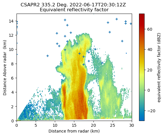
June 17 RHI

We are also interested in the Range-Height Indicator scans provided by CSAPR2 as this cell evolves. The RHI scans will provide a vertical-cross section of the microphysical properties of the storm as it evolves. Finally, this block of code will plot the altitudes and locations of each lightning strike overlaid over the RHI scan. SciPy’s KDTree is used to find the nearest neighbors between the LMA lightning strike locations and the latitude and longitude locations of each gate in the RHI. After the nearest neighbors are found this provides us the altitude and range where the approximate location of the lightning strike would be.

csapr_rhi = pyart.io.read(
    "/Users/rjackson/TRACER-PAWS-NEXRAD-LMA/data/houcsapr2cfrS2.a1.20220617.203012.nc"
)
gatefilter = pyart.filters.GateFilter(csapr_rhi)
gatefilter.exclude_below("normalized_coherent_power", 0.50)

flash_times = np.squeeze(
    np.argwhere(
        np.logical_and(
            lma_ds.flash_time_start.values > np.datetime64("2022-06-17T20:30:00"),
            lma_ds.flash_time_start.values < np.datetime64("2022-06-17T20:31:00"),
        )
    )
)
flash_alts = lma_ds.flash_init_altitude[flash_times]
flash_lons = lma_ds.flash_init_longitude[flash_times]
flash_lats = lma_ds.flash_init_latitude[flash_times]
rhi_lons = csapr_rhi.gate_longitude["data"].flatten()
rhi_lats = csapr_rhi.gate_latitude["data"].flatten()
rhi_alts = csapr_rhi.gate_altitude["data"].flatten()

kdtree_data = np.stack([rhi_lons, rhi_lats], axis=1)
kdtree = KDTree(kdtree_data)
inp_data = np.stack([flash_lons, flash_lats], axis=1)
dist, where_in_rhi = kdtree.query(inp_data)

flash_ranges = csapr_rhi.range["data"][where_in_rhi % csapr_rhi.ngates]
disp = pyart.graph.RadarMapDisplay(csapr_rhi)
disp.plot_rhi("reflectivity", gatefilter=gatefilter)
print(flash_alts.shape)
plt.scatter(flash_ranges / 1e3, flash_alts / 1e3, marker="+")
plt.xlim([0, 30])
plt.ylim([0, 15])

(51,)

(0.0, 15.0)

Active Py-ART Development - Submitting a Pull Request (PR)   Hail Storm Visualization Using Py-ART and Pandas!