Visualizing Severe Weather in Wisconsin#
Motivation#
The Outbreak#
Last Friday (March 31, 2023), a severe weather outbreak impacted a large portion of the Central United States, including the Upper Midwest. There were a total of:
142 tornado reports
368 wind reports, with 7 of those being high wind reports, in excess of 65 knots (~75 mph)
184 hail reports, with 14 of those bing large hail reports, in excess of 2 inches in diameter
Here is a map of the storm reports provided by the National Weather Service:
from IPython.display import IFrame

IFrame(
    src="https://www.spc.noaa.gov/climo/gmf.php?rpt=230331_rpts_filtered",
    width=700,
    height=500,
)
Focusing on Southern Wisconsin#
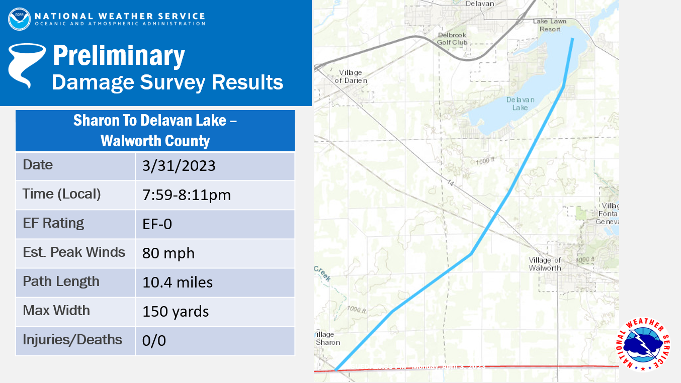
In this blog post, we explore a single area - Walworth County, Wisconsin, which is located in Southeastern Wisconsin. This county is home to Lake Geneva, Wisconsin, a popular tourist destination, especially for those living in the Chicagoland area.
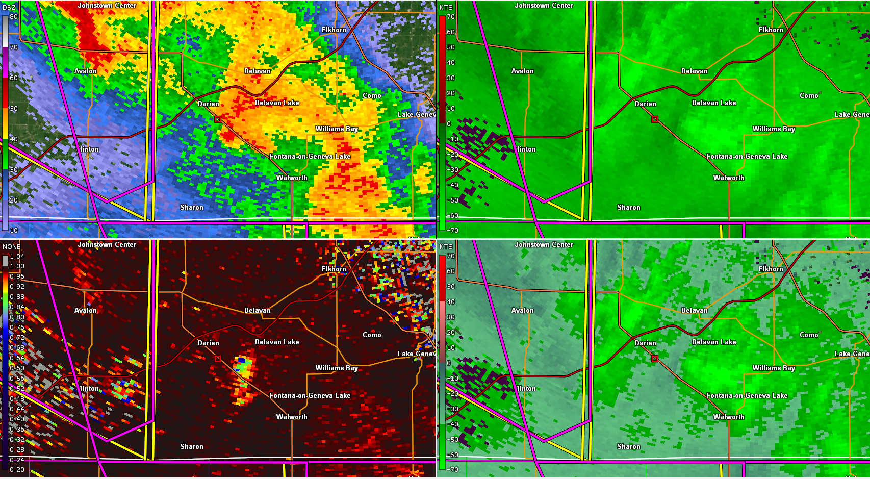
3 confirmed tornadoes moved through Walworth county, with those confirmations from the local National Weather Service (NWS Milwaukee). They also found a considerable amount of wind and hail damage around the area.
NWS Milwaukee assembled an event summary (Link to NWS Event Summary)
which includes the following radar imagery, which was produced using data from their radar and GRLevel software:
Reproducing Event Images#
What if we wanted to reproduce these plots, using free, open-source software, using open data? We can do this using Py-ART. We encourage people check out the Radar Cookbook, which walks through how to get started with the software stack, and details how to work with NEXRAD data, as we are in this case.
The focus here is to build upon the workflow described there, and automate this as much as possible, to enable local NWS offices to easily create post-event evaluation images.
Visualizing the Event#
Imports#
We import a variety of python packages, which can be installed using
conda install -c conda-forge arm_pyart metpy cartopy pandas numpy shapely
from datetime import datetime, timedelta
import warnings

import cartopy.crs as ccrs
import cartopy.feature as cfeature
import cartopy.io.shapereader as shpreader
from cartopy.feature import ShapelyFeature
import fsspec
import matplotlib.pyplot as plt
from metpy.plots import USCOUNTIES
import numpy as np
import pandas as pd
import pyart

warnings.filterwarnings("ignore")
## You are using the Python ARM Radar Toolkit (Py-ART), an open source
## library for working with weather radar data. Py-ART is partly
## supported by the U.S. Department of Energy as part of the Atmospheric
## Radiation Measurement (ARM) Climate Research Facility, an Office of
## Science user facility.
##
## If you use this software to prepare a publication, please cite:
##
##     JJ Helmus and SM Collis, JORS 2016, doi: 10.5334/jors.119
/Users/mgrover/miniforge3/envs/pyart-dev/lib/python3.10/site-packages/tqdm/auto.py:22: TqdmWarning: IProgress not found. Please update jupyter and ipywidgets. See https://ipywidgets.readthedocs.io/en/stable/user_install.html
  from .autonotebook import tqdm as notebook_tqdm
Access the Data#
We start first with some extra map features - in this case, we add interstates to the map (credit to the Census database for the data, and Randy Chase for the code)
Download the Road Data#
I am running this on a Mac, so I used curl, but if you are on a Linux machine you would want to use wget here.
!curl https://www2.census.gov/geo/tiger/TIGER2016/PRIMARYROADS/tl_2016_us_primaryroads.zip --output tl_2016_us_primaryroads.zip
!unzip tl_2016_us_primaryroads.zip
  % Total    % Received % Xferd  Average Speed   Time    Time     Time  Current
                                 Dload  Upload   Total   Spent    Left  Speed
100 25.7M    0 25.7M    0     0  21.0M      0 --:--:--  0:00:01 --:--:-- 21.0M
Archive:  tl_2016_us_primaryroads.zip
 extracting: tl_2016_us_primaryroads.cpg
  inflating: tl_2016_us_primaryroads.dbf
  inflating: tl_2016_us_primaryroads.prj
  inflating: tl_2016_us_primaryroads.shp
  inflating: tl_2016_us_primaryroads.shp.ea.iso.xml
  inflating: tl_2016_us_primaryroads.shp.iso.xml
  inflating: tl_2016_us_primaryroads.shp.xml
  inflating: tl_2016_us_primaryroads.shx
Add the Interstate Date as a feature#
We can add this data as a feature to be used on the maps using Shapely
# Read shape file
reader = shpreader.Reader("./tl_2016_us_primaryroads.shp")
names = []
geoms = []

# Loop through and find the interstates, looking for an I in the full name
for rec in reader.records():
    if rec.attributes["FULLNAME"][0] == "I":
        names.append(rec)
        geoms.append(rec.geometry)

# make interstate feature
interstate_feature = ShapelyFeature(
    geoms, ccrs.PlateCarree(), edgecolor="darkblue", lw=0.5, facecolor="none"
)
Investigate the NEXRAD Data Available#
The NEXRAD data is available through Amazon Web Services (AWS), and we are using the Level2 data, which has been quality controlled to an extent, but has not been fully cleaned (ex. velocity field may still be aliased).
fs = fsspec.filesystem("s3", anon=True)
site = "KMKX"
year = "2023"
month = "04"
day = "01"
hour = "01"
files = sorted(
    fs.glob(
        f"s3://noaa-nexrad-level2/{year}/{month}/{day}/{site}/{site}{year}{month}{day}_{hour}*06"
    )
)
files
['noaa-nexrad-level2/2023/04/01/KMKX/KMKX20230401_010517_V06',
 'noaa-nexrad-level2/2023/04/01/KMKX/KMKX20230401_011057_V06',
 'noaa-nexrad-level2/2023/04/01/KMKX/KMKX20230401_011638_V06',
 'noaa-nexrad-level2/2023/04/01/KMKX/KMKX20230401_012219_V06',
 'noaa-nexrad-level2/2023/04/01/KMKX/KMKX20230401_012759_V06',
 'noaa-nexrad-level2/2023/04/01/KMKX/KMKX20230401_013341_V06',
 'noaa-nexrad-level2/2023/04/01/KMKX/KMKX20230401_013922_V06',
 'noaa-nexrad-level2/2023/04/01/KMKX/KMKX20230401_014502_V06',
 'noaa-nexrad-level2/2023/04/01/KMKX/KMKX20230401_015042_V06',
 'noaa-nexrad-level2/2023/04/01/KMKX/KMKX20230401_015623_V06',
 'noaa-nexrad-level2/2023/04/01/KMKX/KMKX20230401_015928_V06']
Setup our Plotting Functions#
Now that we have our data, we setup a function to process data, which:
Reads the data into a Py-ART radar object
Subset the lowest elevations
Dealias the radial velocity
Plot the velocity
Plot the reflectivity
Save the plot to a file
plot_configuration = {
    "reflectivity": {
        "vmin": -20,
        "vmax": 70,
        "cmap": "pyart_ChaseSpectral",
        "label": "Horizontal Reflectivity (dBZ)",
    },
    "velocity": {
        "vmin": -50,
        "vmax": 50,
        "cmap": "twilight_shifted",
        "label": "Radial Velocity (m/s)",
    },
    "cross_correlation_ratio": {
        "vmin": 0.7,
        "vmax": 1.0,
        "cmap": "pyart_ChaseSpectral",
        "label": "Cross Correlation Ratio",
    },
}
def plot_radar_ppi(
    file,
    left_field="velocity",
    right_field="reflectivity",
    plot_config=plot_configuration,
):
    # Read the radar data
    radar = pyart.io.read_nexrad_archive(f"s3://{file}")

    # Extract the lowest two sweeps - to help with speeding up the data cleaning
    radar = radar.extract_sweeps([0, 1])

    if "velocity" in [left_field, right_field]:
        # Dealias the radial velocities, using a reflectivity threshold to only look at precip regions
        nyq = radar.instrument_parameters["nyquist_velocity"]["data"][0]
        gatefilter = pyart.filters.GateFilter(radar)
        gatefilter.exclude_below("reflectivity", 0)
        vel_dealias = pyart.correct.dealias_region_based(
            radar, nyquist_vel=nyq, centered=True, gatefilter=gatefilter
        )
        radar.add_field("corrected_velocity", vel_dealias, replace_existing=True)

    # Add a subplot for the velocity
    fig = plt.figure(figsize=(14, 8))
    graph = pyart.graph.RadarMapDisplay(radar)

    # Create a plot number to iterate over
    plot_number = 0
    for field in (left_field, right_field):
        # Use the configuration for the field
        config = plot_config[field]

        # Assume 0 sweep (lowest elevation)
        sweep = 0

        # User a new name for the corrected velocity, and use the next sweep
        if (field == "velocity") & (vel_dealias is not None):
            field = "corrected_velocity"
            sweep = 1

        # Plot the first field
        ax = plt.subplot(121 + plot_number, projection=ccrs.PlateCarree())

        # Prepare the title
        title = graph.generate_title(field, 0)
        time = pd.to_datetime(radar.time["units"][-20:])
        time_steps = radar.time["data"]
        index = radar.get_start_end(0)[-1]
        time += timedelta(seconds=time_steps[index])
        central_time = str(time.astimezone("US/Central"))[:-13]
        new_title = f"{title[0:13]} \n {central_time} CDT"
        graph.plot_ppi_map(
            field,
            cmap=config["cmap"],
            sweep=sweep,
            vmin=config["vmin"],
            vmax=config["vmax"],
            ax=ax,
            colorbar_orient="horizontal",
            colorbar_label=config["label"],
            projection=ccrs.PlateCarree(),
        )

        # Add a point near the start of the tornado in Sharon
        ax.scatter(
            -88.7, 42.53, label="Sharon, Wisconsin (Near Start of Tornado)", color="k"
        )

        # Add a point for Delavan Lake, Wisconsin
        ax.scatter(
            -88.6105,
            42.60666,
            label="Delavan Lake, Wisconsin (Near End of Tornado)",
            color="lightgrey",
        )

        # Add the interstates
        ax.add_feature(
            interstate_feature,
            edgecolor="lavenderblush",
            facecolor="None",
            linewidth=2,
            label="Interstate 43",
        )

        # Add the counties
        ax.add_feature(USCOUNTIES, linewidth=0.5)

        # Add gridlines
        gl = ax.gridlines(
            crs=ccrs.PlateCarree(),
            draw_labels=True,
            linewidth=1,
            color="gray",
            alpha=0.3,
            linestyle="--",
        )
        gl.right_labels = False
        gl.top_labels = False

        # Add a label for the interstates
        plt.plot(0, 0, color="lavenderblush", label="Interstate 43")
        plt.xlim(-88.8, -88.2)
        plt.ylim(42.3, 42.9)
        plt.legend(loc="upper right")

        # Add one to the plot number
        plot_number += 1

    plt.title(new_title)
    plt.savefig(f"ppi_velocity_reflectivity_{time}.png", dpi=300)
    plt.show()
    plt.close()
Run our Plotting Functions#
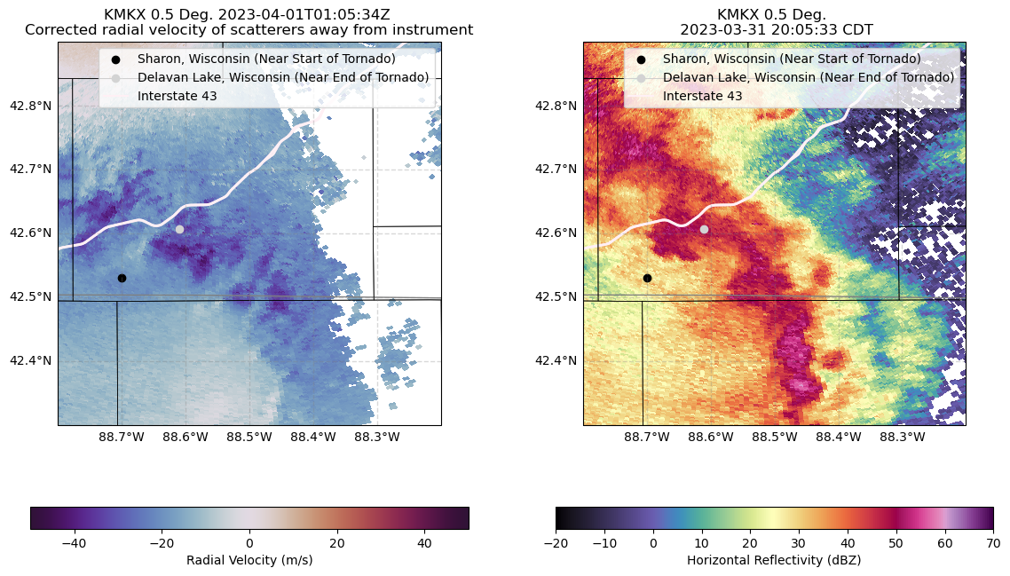
Now that we have our plotting functions, we can apply these to the first volume of our file list, when the NWS identified the Sharon to Delavan Lake tornado
plot_radar_ppi(files[0])
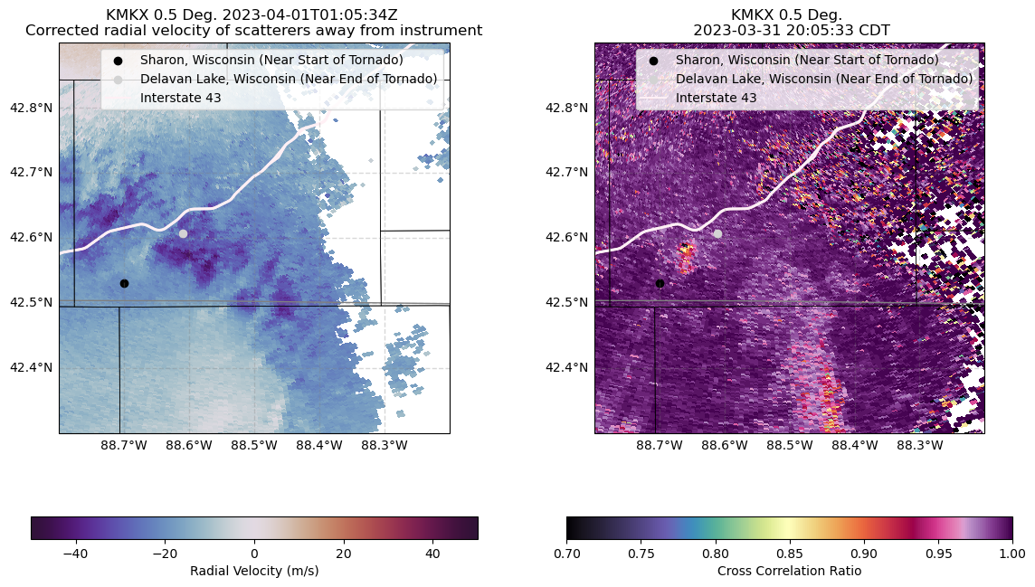
plot_radar_ppi(files[0], right_field="cross_correlation_ratio")
Conclusion#
Within this post, we examined how to use data from the National Weather Service to identify tornado signatures, and create a flexible plotting function to visualize its path. We even added interstates for reference!
We hope that this will be applicable to NWS offices interested in making colorblind-friendly maps of severe weather events, and automate the data selection and visualization process (where possible).