Note
Go to the end to download the full example code.
Consolidation of Data Sources#
This example shows how to use ACT to combine multiple datasets to support ARM’s AMF3.
Downloading: 1M4
Downloading ctd24293.00m
Downloading ctd24293.01m
Downloading ctd24293.02m
Downloading ctd24293.03m
Downloading ctd24293.04m
Downloading ctd24293.05m
Downloading ctd24293.06m
Downloading ctd24293.07m
Downloading ctd24293.08m
Downloading ctd24293.09m
Downloading ctd24293.10m
Downloading ctd24293.11m
Downloading ctd24293.12m
Downloading ctd24293.13m
Downloading ctd24293.14m
Downloading ctd24293.15m
Downloading ctd24293.16m
Downloading ctd24293.17m
Downloading ctd24293.18m
Downloading ctd24293.19m
Downloading ctd24293.20m
Downloading ctd24293.21m
Downloading ctd24293.22m
Downloading ctd24293.23m
Downloading ctd24294.00m
Downloading ctd24294.01m
Downloading ctd24294.02m
Downloading ctd24294.03m
Downloading ctd24294.04m
Downloading ctd24294.05m
Downloading ctd24294.06m
Downloading ctd24294.07m
Downloading ctd24294.08m
Downloading ctd24294.09m
Downloading ctd24294.10m
Downloading ctd24294.11m
Downloading ctd24294.12m
Downloading ctd24294.13m
Downloading ctd24294.14m
Downloading ctd24294.15m
Downloading ctd24294.16m
Downloading ctd24294.17m
Downloading ctd24294.18m
Downloading ctd24294.19m
Downloading ctd24294.20m
Downloading ctd24294.21m
Downloading ctd24294.22m
Downloading ctd24294.23m
Downloading ctd24295.00m
Downloading ctd24295.01m
Downloading ctd24295.02m
Downloading ctd24295.03m
Downloading ctd24295.04m
Downloading ctd24295.05m
Downloading ctd24295.06m
Downloading ctd24295.07m
Downloading ctd24295.08m
Downloading ctd24295.09m
Downloading ctd24295.10m
Downloading ctd24295.11m
Downloading ctd24295.12m
Downloading ctd24295.13m
Downloading ctd24295.14m
Downloading ctd24295.15m
Downloading ctd24295.16m
Downloading ctd24295.17m
Downloading ctd24295.18m
Downloading ctd24295.19m
Downloading ctd24295.20m
Downloading ctd24295.21m
Downloading ctd24295.22m
Downloading ctd24295.23m
Downloading ctd24296.00m
Downloading ctd24296.01m
Downloading ctd24296.02m
Downloading ctd24296.03m
Downloading ctd24296.04m
Downloading ctd24296.05m
Downloading ctd24296.06m
Downloading ctd24296.07m
Downloading ctd24296.08m
Downloading ctd24296.09m
Downloading ctd24296.10m
Downloading ctd24296.11m
Downloading ctd24296.12m
Downloading ctd24296.13m
Downloading ctd24296.14m
Downloading ctd24296.15m
Downloading ctd24296.16m
Downloading ctd24296.17m
Downloading ctd24296.18m
Downloading ctd24296.19m
Downloading ctd24296.20m
Downloading ctd24296.21m
Downloading ctd24296.22m
Downloading ctd24296.23m
Downloading ctd24297.00m
Downloading ctd24297.01m
Downloading ctd24297.02m
Downloading ctd24297.03m
Downloading ctd24297.04m
Downloading ctd24297.05m
Downloading ctd24297.06m
Downloading ctd24297.07m
Downloading ctd24297.08m
Downloading ctd24297.09m
Downloading ctd24297.10m
Downloading ctd24297.11m
Downloading ctd24297.12m
Downloading ctd24297.13m
Downloading ctd24297.14m
Downloading ctd24297.15m
Downloading ctd24297.16m
Downloading ctd24297.17m
Downloading ctd24297.18m
Downloading ctd24297.19m
Downloading ctd24297.20m
Downloading ctd24297.21m
Downloading ctd24297.22m
Downloading ctd24297.23m
Downloading ctd24298.00m
Downloading ctd24298.01m
Downloading ctd24298.02m
Downloading ctd24298.03m
Downloading ctd24298.04m
Downloading ctd24298.05m
Downloading ctd24298.06m
Downloading ctd24298.07m
Downloading ctd24298.08m
Downloading ctd24298.09m
Downloading ctd24298.10m
Downloading ctd24298.11m
Downloading ctd24298.12m
Downloading ctd24298.13m
Downloading ctd24298.14m
Downloading ctd24298.15m
Downloading ctd24298.16m
Downloading ctd24298.17m
Downloading ctd24298.18m
Downloading ctd24298.19m
Downloading ctd24298.20m
Downloading ctd24298.21m
Downloading ctd24298.22m
Downloading ctd24298.23m
[DOWNLOADING] bnfmetM1.b1.20241019.000000.cdf
[DOWNLOADING] bnfmetM1.b1.20241020.000000.cdf
[DOWNLOADING] bnfmetM1.b1.20241021.000000.cdf
[DOWNLOADING] bnfmetM1.b1.20241022.000000.cdf
[DOWNLOADING] bnfmetM1.b1.20241023.000000.cdf
[DOWNLOADING] bnfmetM1.b1.20241024.000000.cdf

If you use these data to prepare a publication, please cite:

Kyrouac, J., Shi, Y., & Tuftedal, M. Surface Meteorological Instrumentation
(MET), 2024-10-19 to 2024-10-24, Bankhead National Forest, AL, USA; Long-term
Mobile Facility (BNF), Bankhead National Forest, AL, AMF3 (Main Site) (M1).
Atmospheric Radiation Measurement (ARM) User Facility.
https://doi.org/10.5439/1786358

[DOWNLOADING] bnfaoso3M1.b1.20241019.000000.nc
[DOWNLOADING] bnfaoso3M1.b1.20241020.000000.nc
[DOWNLOADING] bnfaoso3M1.b1.20241021.000001.nc
[DOWNLOADING] bnfaoso3M1.b1.20241022.000000.nc
[DOWNLOADING] bnfaoso3M1.b1.20241023.000000.nc

If you use these data to prepare a publication, please cite:

Sedlacek, A., Hayes, C., Springston, S., Koontz, A., & Trojanowski, R. Ozone
Monitor (AOSO3), 2024-10-19 to 2024-10-24, Bankhead National Forest, AL, USA;
Long-term Mobile Facility (BNF), Bankhead National Forest, AL, AMF3 (Main Site)
(M1). Atmospheric Radiation Measurement (ARM) User Facility.
https://doi.org/10.5439/1346692

[DOWNLOADING] bnfaossmpsM1.b1.20241019.000459.nc
[DOWNLOADING] bnfaossmpsM1.b1.20241020.000459.nc
[DOWNLOADING] bnfaossmpsM1.b1.20241021.000459.nc
[DOWNLOADING] bnfaossmpsM1.b1.20241022.000459.nc
[DOWNLOADING] bnfaossmpsM1.b1.20241023.000459.nc

If you use these data to prepare a publication, please cite:

Singh, A., Kuang, C., Howie, J., Salwen, C., & Hayes, C. Scanning mobility
particle sizer (AOSSMPS), 2024-10-19 to 2024-10-24, Bankhead National Forest,
AL, USA; Long-term Mobile Facility (BNF), Bankhead National Forest, AL, AMF3
(Main Site) (M1). Atmospheric Radiation Measurement (ARM) User Facility.
https://doi.org/10.5439/1476898
import os
from datetime import datetime
import matplotlib.pyplot as plt
import numpy as np
import act
# Get Surface Meteorology data from the ASOS stations
station = '1M4'
time_window = [datetime(2024, 10, 19), datetime(2024, 10, 24)]
ds_asos = act.discovery.get_asos_data(time_window, station=station, regions='AL')[station]
ds_asos = ds_asos.where(~np.isnan(ds_asos.tmpf), drop=True)
ds_asos['tmpf'].attrs['units'] = 'degF'
ds_asos.utils.change_units(variables='tmpf', desired_unit='degC', verbose=True)
# Pull EPA data from AirNow
# You need an account and token from https://docs.airnowapi.org/ first
airnow_token = os.getenv('AIRNOW_API')
if airnow_token is not None and len(airnow_token) > 0:
latlon = '-87.453,34.179,-86.477,34.787'
ds_airnow = act.discovery.get_airnow_bounded_obs(
airnow_token, '2024-10-19T00', '2024-10-24T23', latlon, 'OZONE,PM25', data_type='B'
)
ds_airnow = act.utils.convert_2d_to_1d(ds_airnow, parse='sites')
sites = ds_airnow['sites'].values
airnow = True
# Get NOAA PSL Data from Courtland
results = act.discovery.download_noaa_psl_data(
site='ctd', instrument='Temp/RH', startdate='20241019', enddate='20241024'
)
ds_noaa = act.io.read_psl_surface_met(results)
# Place your username and token here
username = os.getenv('ARM_USERNAME')
token = os.getenv('ARM_PASSWORD')
# Download ARM data for the MET, OZONE, and SMPS
if username is not None and token is not None and len(username) > 1:
# Example to show how easy it is to download ARM data if a username/token are set
results = act.discovery.download_arm_data(
username, token, 'bnfmetM1.b1', '2024-10-19', '2024-10-24'
)
ds_arm = act.io.arm.read_arm_netcdf(results)
results = act.discovery.download_arm_data(
username, token, 'bnfaoso3M1.b1', '2024-10-19', '2024-10-24'
)
ds_o3 = act.io.arm.read_arm_netcdf(results, cleanup_qc=True)
ds_o3.qcfilter.datafilter('o3', rm_assessments=['Suspect', 'Bad'], del_qc_var=False)
results = act.discovery.download_arm_data(
username, token, 'bnfaossmpsM1.b1', '2024-10-19', '2024-10-24'
)
ds_smps = act.io.arm.read_arm_netcdf(results)
# Set up display and plot all the data
display = act.plotting.TimeSeriesDisplay(
{'ASOS': ds_asos, 'ARM': ds_arm, 'EPA': ds_airnow, 'NOAA': ds_noaa, 'ARM_O3': ds_o3},
figsize=(12, 10),
subplot_shape=(3,),
)
# Plot surface temperature from ASOS, NOAA, and ARM sites
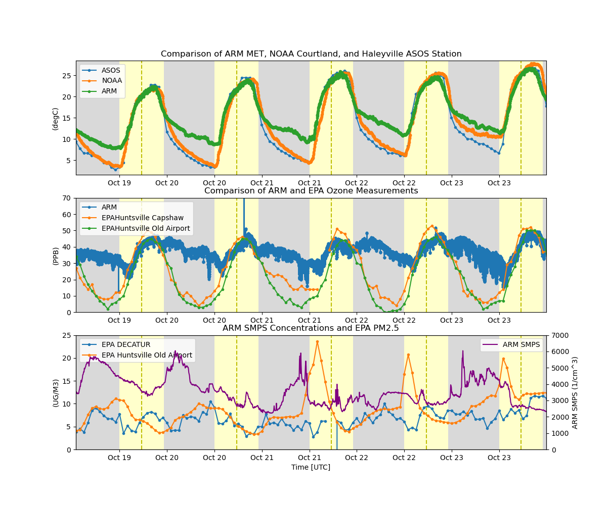
title = 'Comparison of ARM MET, NOAA Courtland, and Haleyville ASOS Station'
display.plot('tmpf', dsname='ASOS', label='ASOS', subplot_index=(0,))
display.plot('Temperature', dsname='NOAA', label='NOAA', subplot_index=(0,))
display.plot('temp_mean', dsname='ARM', label='ARM', subplot_index=(0,), set_title=title)
display.day_night_background(dsname='ARM', subplot_index=(0,))
# Plot ARM and EPA Ozone data
title = 'Comparison of ARM and EPA Ozone Measurements'
display.plot('o3', dsname='ARM_O3', label='ARM', subplot_index=(1,))
if airnow:
display.plot('OZONE_sites_1', dsname='EPA', label='EPA' + sites[1], subplot_index=(1,))
display.plot(
'OZONE_sites_2',
dsname='EPA',
label='EPA' + sites[2],
subplot_index=(1,),
set_title=title,
)
display.set_yrng([0, 70], subplot_index=(1,))
display.day_night_background(dsname='ARM', subplot_index=(1,))
# Plot ARM SMPS Concentrations and EPA PM2.5 data on different axes
title = 'ARM SMPS Concentrations and EPA PM2.5'
if airnow:
display.plot('PM2.5_sites_0', dsname='EPA', label='EPA ' + sites[0], subplot_index=(2,))
display.plot(
'PM2.5_sites_2',
dsname='EPA',
label='EPA ' + sites[2],
subplot_index=(2,),
set_title=title,
)
display.set_yrng([0, 25], subplot_index=(2,))
ax2 = display.axes[2].twinx()
ax2.plot(ds_smps['time'], ds_smps['total_N_conc'], label='ARM SMPS', color='purple')
ax2.set_ylabel('ARM SMPS (' + ds_smps['total_N_conc'].attrs['units'] + ')')
ax2.set_ylim([0, 7000])
ax2.legend(loc=1)
display.day_night_background(dsname='ARM', subplot_index=(2,))
# Set legends
for ax in display.axes:
ax.legend(loc=2)
plt.show()
else:
pass
Total running time of the script: (1 minutes 1.947 seconds)