Planetary Boundary Layer Height Profile Fit Retrievals

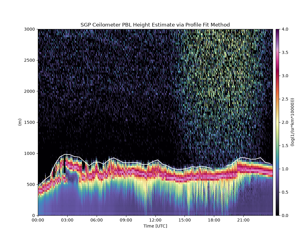
This example shows how to estimate the planetary boundary layer height via a Profile Method scheme, where a backscatter profile is fit to an idealized profile via an error function using non-linear least-squares optimization.

Author: Joe O’Brien

from arm_test_data import DATASETS

import act

# Read Ceilometer data for an example
filename_ceil = DATASETS.fetch('sgpceilC1.b1.20190101.000000.nc')
ds = act.io.arm.read_arm_netcdf(filename_ceil)

# Estimate PBL Height via a Profile Method
ds = act.retrievals.pbl_lidar.calculate_profile_fit_pbl(ds, parm="backscatter")
# Apply the ceilometer correction to the backscatter variable for plotting
# Note - after the PBL Height retrieval.
ds = act.corrections.correct_ceil(ds, var_name='backscatter')

# Plot the pbl height estimates
display = act.plotting.TimeSeriesDisplay(ds, subplot_shape=(1,), figsize=(10, 8))

# plot the CL backscatter before overlaying the Gradient Method PBL Height
display.plot(
    'backscatter',
    subplot_index=(0,),
    cmap='ChaseSpectral',
    vmin=0,
    vmax=4,
    set_title='SGP Ceilometer PBL Height Estimate via Profile Fit Method',
)

# overlay the PBL Height estimate, compute ~10min temporal averages
display.axes[0].plot(
    ds['time'].resample(time="30min").mean().values,
    ds['pbl_profile_fit'].resample(time="30min").mean().values,
    color='white',
)
# shorten the range
display.set_yrng([0, 3000], subplot_index=(0,))