Propagating quality control through a resample

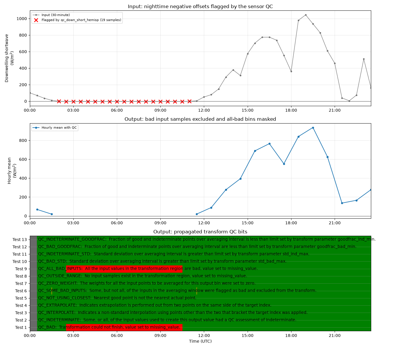
Shortwave irradiance should not be negative. This example uses a real ARM surface-radiation file in which the downwelling shortwave sensor reports small negative nighttime offsets. The datastream’s fail_min QC test flags those samples as bad.

The flagged samples are excluded while the data are transformed to an hourly time base. The transformed output QC records which hourly bins lost some or all of their input. The all-missing interval around 02:30 UTC is intentional: every input contributing to that hourly bin failed the source QC test, so the transform marks it QC_ALL_BAD_INPUTS and leaves it missing. The three-panel figure shows the input flags, the cleaned transformed output, and the propagated output QC bitfield.

flag_meanings: [np.str_('Value is equal to missing_value.'), 'Value is less than the fail_min.', 'Value is greater than the fail_max.']
qc assessment excluded = Bad

Input range:              -3.3 to 1044.2 W/m^2
Bad output bins masked:   9 of 24

import matplotlib.pyplot as plt
import numpy as np
import xarray as xr
from arm_test_data import DATASETS

import act

filename = DATASETS.fetch('sgpsebsE39.b1.20230601.000000.cdf')
ds = act.io.arm.read_arm_netcdf(filename, cleanup_qc=True)

var_name = 'down_short_hemisp'
qc_var_name = 'qc_' + var_name

# Pass the QC assessment to exclude; bin_average resolves the matching bitmask
# from the QC variable's CF flag metadata.
qc_da = ds[qc_var_name]
qc_mask = 'Bad'

print(f'flag_meanings: {qc_da.attrs["flag_meanings"]}')
print(f'qc assessment excluded = {qc_mask}')

# Use hourly centers at :30 so the output cells run from each hour to the next.
target = act.transform.make_coord('2023-06-01T00:30', '2023-06-01T23:30', '1h', name='time')
half_hour = np.timedelta64(30, 'm')
output_bounds = np.column_stack((target.values - half_hour, target.values + half_hour))

# Flagged samples are excluded, and the output QC records which bins lost
# some or all of their input.
filtered, filtered_qc = act.transform.bin_average(
    ds[var_name],
    target,
    dim='time',
    qc=qc_da,
    qc_mask=qc_mask,
    output_bounds=output_bounds,
)

bad_masks = [
    int(mask)
    for mask, assessment in zip(qc_da.attrs['flag_masks'], qc_da.attrs['flag_assessments'])
    if assessment == qc_mask
]
flagged_input = np.zeros(qc_da.shape, dtype=bool)
for mask in bad_masks:
    flagged_input |= (qc_da.values & mask).astype(bool)

# Assemble the transformed data and QC, then run ACT's standard cleanup. The
# transform uses -9999 as its output missing-value sentinel. cleanup() handles
# the QC metadata; explicitly decoding that sentinel keeps it from skewing the
# output plot while preserving the QC variable for the block plot.
output_ds = xr.Dataset({filtered.name: filtered, filtered_qc.name: filtered_qc})
output_ds[filtered.name].attrs['ancillary_variables'] = filtered_qc.name
output_ds.clean.cleanup()
output_ds[filtered.name] = output_ds[filtered.name].where(output_ds[filtered.name] != -9999)

print(
    f'\nInput range:              '
    f'{float(np.nanmin(ds[var_name])):.1f} to {float(np.nanmax(ds[var_name])):.1f} W/m^2'
)
print(f'Bad output bins masked:   {int(np.isnan(output_ds[var_name]).sum())} of {filtered.size}')

# Plot input values and bad input samples, transformed output, and propagated
# transform QC in one shared figure.
display = act.plotting.TimeSeriesDisplay(
    {'Input': ds, 'Transformed': output_ds},
    figsize=(14, 12),
    subplot_shape=(3,),
)

display.plot(
    var_name,
    dsname='Input',
    subplot_index=(0,),
    label='Input (30-minute)',
    color='0.45',
    marker='o',
    ms=3,
    lw=1,
)
display.axes[0].plot(
    ds['time'].values[flagged_input],
    ds[var_name].values[flagged_input],
    'rx',
    ms=8,
    mew=2,
    label=f'Flagged by {qc_var_name} ({flagged_input.sum()} samples)',
)
display.axes[0].axhline(0, color='0.3', lw=0.8)
display.axes[0].set_ylabel('Downwelling shortwave\n(W/m$^2$)')
display.axes[0].set_title('Input: nighttime negative offsets flagged by the sensor QC')
display.axes[0].legend(loc='upper left', fontsize=8)
display.axes[0].grid(alpha=0.3)

display.plot(
    var_name,
    dsname='Transformed',
    subplot_index=(1,),
    label='Hourly mean with QC',
    color='tab:blue',
    marker='o',
    ms=4,
    lw=1.5,
)
display.axes[1].axhline(0, color='0.3', lw=0.8)
display.axes[1].set_ylabel('Hourly mean\n(W/m$^2$)')
display.axes[1].set_title('Output: bad input samples excluded and all-bad bins masked')
display.axes[1].legend(loc='upper left', fontsize=8)
display.axes[1].grid(alpha=0.3)

display.qc_flag_block_plot(
    var_name,
    dsname='Transformed',
    subplot_index=(2,),
    ylabel='Output QC flags',
)
display.axes[2].set_title('Output: propagated transform QC bits')
display.axes[2].set_xlabel('Time (UTC)')
display.axes[2].grid(alpha=0.3, axis='y')

display.fig.tight_layout()
plt.show()

ds.close()