Resample a datastream onto a coarser time base

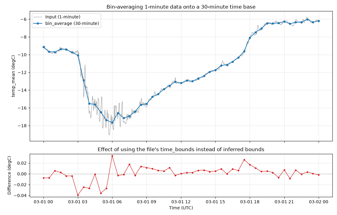
This example bin-averages 1-minute ARM surface meteorology data onto a 30-minute time base using act.transform.bin_average, and shows how the file’s CF time_bounds variable is used to weight each input sample by how much of its measurement interval overlaps each output bin.

Input samples:  1440
Output samples: 49
Max difference from using declared bounds: 0.039333 degC
Output QC values present: [0]

import matplotlib.pyplot as plt
import numpy as np
from arm_test_data import DATASETS

import act

# Read a day of 1-minute surface meteorology data from the ARM test data
# collection, so no ARM credentials are needed to run this example.
filename = DATASETS.fetch('gucmetM1.b1.20230301.000000.cdf')
ds = act.io.arm.read_arm_netcdf(filename, cleanup_qc=True)

var_name = 'temp_mean'

# Build the target coordinate. make_coord accepts datetime-like endpoints with
# a pandas frequency string, and returns a DataArray we can transform onto.
target = act.transform.make_coord('2023-03-01', '2023-03-02', '30min', name='time')

# Bin-average onto the coarser coordinate. Each transform returns a
# (result, result_qc) tuple; result_qc describes how each output point was made.
result, result_qc = act.transform.bin_average(ds[var_name], target, dim='time')

# This file carries a CF time_bounds variable saying which interval each sample
# summarizes. Passing it as input_bounds means samples straddling an output bin
# edge are split across both bins rather than assigned entirely to one.
result_bounds, _ = act.transform.bin_average(
    ds[var_name], target, dim='time', input_bounds=ds['time_bounds'].values
)

# Plot the original data against both results.
fig, (ax0, ax1) = plt.subplots(
    2, 1, figsize=(11, 7), sharex=True, gridspec_kw={'height_ratios': [3, 1]}
)

ax0.plot(ds['time'].values, ds[var_name].values, color='0.6', lw=0.8, label='Input (1-minute)')
ax0.plot(
    result['time'].values,
    result.values,
    color='tab:blue',
    marker='o',
    ms=4,
    lw=1.5,
    label='bin_average (30-minute)',
)
ax0.set_ylabel(f'{var_name} ({ds[var_name].attrs["units"]})')
ax0.set_title('Bin-averaging 1-minute data onto a 30-minute time base')
ax0.legend(loc='upper left')
ax0.grid(alpha=0.3)

# The difference between inferring bounds from midpoints and using the file's
# declared bounds is small for evenly spaced data, but it is not zero.
difference = result_bounds.values - result.values
ax1.axhline(0, color='0.7', lw=0.8)
ax1.plot(result['time'].values, difference, color='tab:red', marker='.', lw=1)
ax1.set_ylabel('Difference (degC)')
ax1.set_xlabel('Time (UTC)')
ax1.set_title('Effect of using the file\'s time_bounds instead of inferred bounds')
ax1.grid(alpha=0.3)

print(f'Input samples:  {ds.sizes["time"]}')
print(f'Output samples: {result.sizes["time"]}')
print(f'Max difference from using declared bounds: {np.abs(difference).max():.6f} degC')
print(f'Output QC values present: {sorted(set(result_qc.values.tolist()))}')

fig.tight_layout()
plt.show()

ds.close()