Comparing bin_average, interpolate, and subsample

This example compares the three transforms on temperature and a present-weather code. The target is offset by 30 seconds from the input timestamps, so no target point matches an input sample exactly.

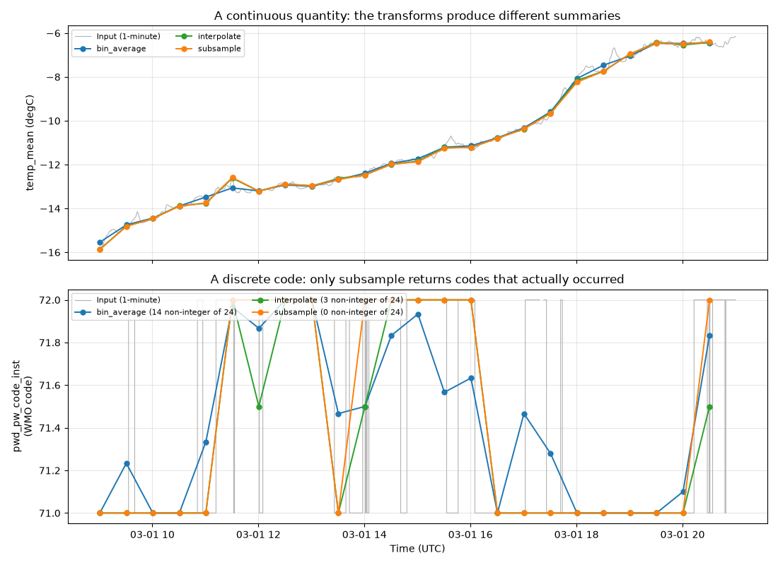
temp_mean            bin_average  mean=-11.1677  step-to-step std=0.3391
temp_mean            interpolate  mean=-11.2030  step-to-step std=0.4407
temp_mean            subsample    mean=-11.2099  step-to-step std=0.4317
pwd_pw_code_inst     bin_average  non-integer outputs= 14/24  unique=[71.         71.1        71.23333333 71.28       71.33333333]
pwd_pw_code_inst     interpolate  non-integer outputs=  3/24  unique=[71.  71.5 72. ]
pwd_pw_code_inst     subsample    non-integer outputs=  0/24  unique=[71. 72.]

import matplotlib.pyplot as plt
import numpy as np
from arm_test_data import DATASETS

import act

filename = DATASETS.fetch('gucmetM1.b1.20230301.000000.cdf')
ds = act.io.arm.read_arm_netcdf(filename, cleanup_qc=True)

# A 30-minute target over a 12-hour window, offset from the input grid.
target = act.transform.make_coord(
    '2023-03-01T09:00:30', '2023-03-01T21:00:00', '30min', name='time'
)
window = slice('2023-03-01T09:00:00', '2023-03-01T21:00:00')

# Apply each transform to the same target coordinate.
transforms = ['bin_average', 'interpolate', 'subsample']
colors = {'bin_average': 'tab:blue', 'interpolate': 'tab:green', 'subsample': 'tab:orange'}

fig, (ax0, ax1) = plt.subplots(2, 1, figsize=(11, 8), sharex=True)

# --- A continuous quantity: temperature ---------------------------------------
# Bin-averaging summarizes the whole interval, so it smooths the 1-minute noise.
# Interpolate and subsample each report a single instant, so they follow it.
var_name = 'temp_mean'
sub = ds[var_name].sel(time=window)
ax0.plot(sub['time'].values, sub.values, color='0.7', lw=0.8, label='Input (1-minute)')

for name in transforms:
    result, _ = getattr(act.transform, name)(ds[var_name], target, dim='time')
    ax0.plot(
        result['time'].values,
        result.values,
        marker='o',
        ms=5,
        lw=1.4,
        color=colors[name],
        label=name,
    )
    # Spread of successive differences: a proxy for how much noise survives.
    roughness = float(np.std(np.diff(result.values)))
    print(
        f'{var_name:20s} {name:12s} mean={float(result.mean()):8.4f}  '
        f'step-to-step std={roughness:.4f}'
    )

ax0.set_ylabel(f'{var_name} ({ds[var_name].attrs["units"]})')
ax0.set_title('A continuous quantity: the transforms produce different summaries')
ax0.legend(loc='upper left', fontsize=8, ncol=2)
ax0.grid(alpha=0.3)

# --- A discrete quantity: present-weather code -------------------------------
# These are categorical WMO codes, not magnitudes. Code 71 and code 72 describe
# different conditions; 71.5 describes nothing. Averaging invents such values,
# and so does interpolating between two different codes. Only subsample is
# guaranteed to return a code that actually occurred.
code_name = 'pwd_pw_code_inst'
sub_code = ds[code_name].sel(time=window)
ax1.plot(
    sub_code['time'].values,
    sub_code.values,
    color='0.7',
    lw=0.8,
    drawstyle='steps-post',
    label='Input (1-minute)',
)

for name in transforms:
    result, _ = getattr(act.transform, name)(ds[code_name], target, dim='time')
    values = result.values
    n_invented = int((values != np.round(values)).sum())
    ax1.plot(
        result['time'].values,
        values,
        marker='o',
        ms=5,
        lw=1.4,
        color=colors[name],
        label=f'{name} ({n_invented} non-integer of {values.size})',
    )
    print(
        f'{code_name:20s} {name:12s} non-integer outputs={n_invented:3d}/{values.size}  '
        f'unique={np.unique(values)[:5]}'
    )

ax1.set_ylabel(f'{code_name}\n(WMO code)')
ax1.set_xlabel('Time (UTC)')
ax1.set_title('A discrete code: only subsample returns codes that actually occurred')
ax1.legend(loc='upper left', fontsize=8, ncol=2)
ax1.grid(alpha=0.3)

fig.tight_layout()
plt.show()

ds.close()