Note
Go to the end to download the full example code.
Convective-Stratiform classification#
This example shows how to use the updated convective stratiform classifcation algorithm. We show 3 examples, a summer convective example, an example from Hurricane Ian, and an example from a winter storm.
print(__doc__)

# Author: Laura Tomkins (lmtomkin@ncsu.edu)
# License: BSD 3 clause


import cartopy.crs as ccrs
import matplotlib.colors as mcolors
import matplotlib.pyplot as plt
import numpy as np

import pyart
How the algorithm works#
This first section describes how the convective-stratiform algorithm works (see references for full details). This
algorithm is a feature detection algorithm and classifies fields as “convective” or “stratiform”. The algorithm is
designed to detect features in a reflectivity field but can also detect features in fields such as rain rate or
snow rate. In this section we describe the steps of the convective stratiform algorithm and the variables used in
the function.
The first step of the algorithm calculates a background average of the field with a circular footprint using a radius
provided by bkg_rad_km. A larger radius will yield a smoother field. The radius needs to be at least double the
grid spacing, but we recommend at least three times the grid spacing. If using reflectivity, dB_averaging should be set
to True to convert reflectivity to linear Z before averaging, False for rescaled fields such as rain or snow rate.
calc_thres determines the minimum fraction of a circle that is considered in the background average calculation
(default is 0.75, so the points along the edges where there is less than 75% of a full circle of data,
the algorithm is not run).
Once the background average has been calculated, the original field is compared to the background average. In
order for points to be considered “convective cores” they must exceed the background value by a certain value or
simply be greater than the always_core_thres. This value is determined by either a cosine scheme, or a scalar
value (i.e. the reflectivity value must be X times the background value (multiplier; use_addition=False),
or X greater than the background value (use_addition=True) where X is the scalar_diff).
use_cosine determines if a cosine scheme or scalar scheme is to be used. If use_cosine is True,
then the max_diff and zero_diff_cos_val come into use. These values define the cosine scheme that is used to
determine the minimum difference between the background and reflectivity value in order for a core to be
identified. max_diff is the maximum difference between the field and the background for a core to be identified,
or where the cosine function crosses the y-axis. The zero_diff_cos_val is where the difference between the field
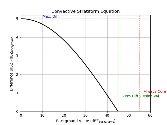
and the background is zero, or where the cosine function crosses the x-axis. Note, if
always_core_thres < zero_diff_cos_val, zero_diff_cos_val only helps define the shape of the cosine curve and
all values greater than always_core_thres will be considered a convective core. If
always_core_thres > zero_diff_cos_val then all values greater than zero_diff_cos_val will be considered a
convective core. We plot some examples of the schemes below:
Example of the cosine scheme:
pyart.graph.plot_convstrat_scheme(
    always_core_thres=30, use_cosine=True, max_diff=5, zero_diff_cos_val=45
)
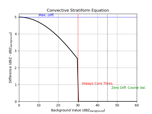
when zero_diff_cos_val is greater than always_core_thres, the difference becomes zero at the zero_diff_cos_val
pyart.graph.plot_convstrat_scheme(
    always_core_thres=55, use_cosine=True, max_diff=5, zero_diff_cos_val=45
)
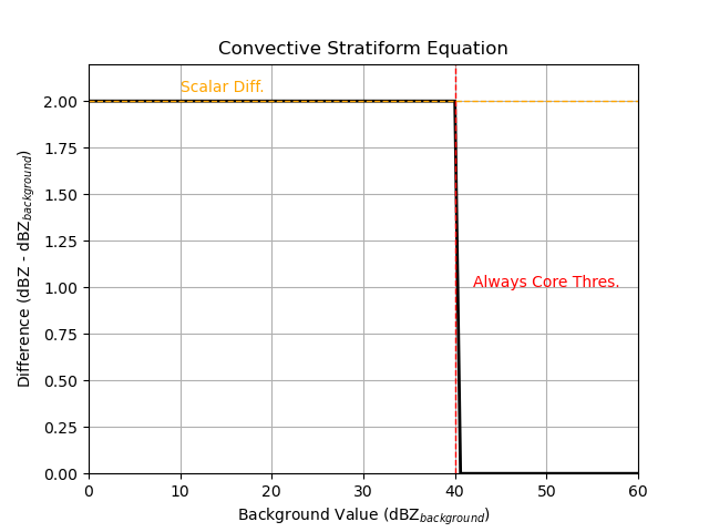
alternatively, we can use a simpler scalar difference instead of a cosine scheme
pyart.graph.plot_convstrat_scheme(
    always_core_thres=40,
    use_cosine=False,
    max_diff=None,
    zero_diff_cos_val=None,
    use_addition=True,
    scalar_diff=2,
)
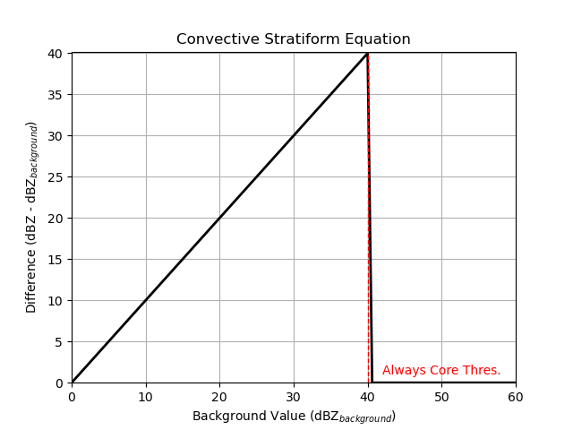
if you are interested in picking up weak features, you can also use the scalar difference as a multiplier instead, so very weak features do not have to be that different from the background to be classified as convective.
pyart.graph.plot_convstrat_scheme(
    always_core_thres=40,
    use_cosine=False,
    max_diff=None,
    zero_diff_cos_val=None,
    use_addition=False,
    scalar_diff=2,
)
Once the cores are identified, there is an option to remove speckles (remove_small_objects) smaller than a given
size (min_km2_size).
After the convective cores are identified, We then incorporate convective radii using
val_for_max_conv_rad and max_conv_rad_km. The convective radii act as a dilation and are used to classify
additional points around the cores as convective that may not have been identified previously. The
val_for_max_conv_rad is the value where the maximum convective radius is applied and the max_conv_rad_km is the
maximum convective radius. Values less than the val_for_max_conv_rad are assigned a convective radius using a step
function.
Finally, the points are classified as NOSFCECHO (threshold set with min_dBZ_used; 0), WEAKECHO (threshold set with
weak_echo_thres; 3), SF (stratiform; 1), CONV (convective; 2).
Examples#
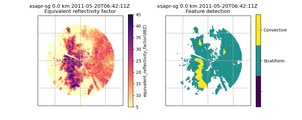
Classification of summer convective example
Our first example classifies echo from a summer convective event. We use a cosine scheme to classify the convective points.
# Now let's do a classification with our parameters
# read in file
filename = pyart.testing.get_test_data("swx_20120520_0641.nc")
radar = pyart.io.read(filename)

# extract the lowest sweep
radar = radar.extract_sweeps([0])

# interpolate to grid
grid = pyart.map.grid_from_radars(
    (radar,),
    grid_shape=(1, 201, 201),
    grid_limits=((0, 10000), (-50000.0, 50000.0), (-50000.0, 50000.0)),
    fields=["reflectivity_horizontal"],
)

# get dx dy
dx = grid.x["data"][1] - grid.x["data"][0]
dy = grid.y["data"][1] - grid.y["data"][0]

# convective stratiform classification
convsf_dict = pyart.retrieve.conv_strat_yuter(
    grid,
    dx,
    dy,
    refl_field="reflectivity_horizontal",
    always_core_thres=40,
    bkg_rad_km=20,
    use_cosine=True,
    max_diff=5,
    zero_diff_cos_val=55,
    weak_echo_thres=10,
    max_conv_rad_km=2,
)

# add to grid object
# mask zero values (no surface echo)
convsf_masked = np.ma.masked_equal(convsf_dict["feature_detection"]["data"], 0)
# mask 3 values (weak echo)
convsf_masked = np.ma.masked_equal(convsf_masked, 3)
# add dimension to array to add to grid object
convsf_dict["feature_detection"]["data"] = convsf_masked
# add field
grid.add_field("convsf", convsf_dict["feature_detection"], replace_existing=True)

# create plot using GridMapDisplay
# plot variables
display = pyart.graph.GridMapDisplay(grid)
magma_r_cmap = plt.get_cmap("magma_r")
ref_cmap = mcolors.LinearSegmentedColormap.from_list(
    "ref_cmap", magma_r_cmap(np.linspace(0, 0.9, magma_r_cmap.N))
)
projection = ccrs.AlbersEqualArea(
    central_latitude=radar.latitude["data"][0],
    central_longitude=radar.longitude["data"][0],
)

# plot
plt.figure(figsize=(10, 4))
ax1 = plt.subplot(1, 2, 1, projection=projection)
display.plot_grid(
    "reflectivity_horizontal",
    vmin=5,
    vmax=45,
    cmap=ref_cmap,
    transform=ccrs.PlateCarree(),
    ax=ax1,
)
ax2 = plt.subplot(1, 2, 2, projection=projection)
display.plot_grid(
    "convsf",
    vmin=0,
    vmax=2,
    cmap=plt.get_cmap("viridis", 3),
    ax=ax2,
    transform=ccrs.PlateCarree(),
    ticks=[1 / 3, 1, 5 / 3],
    ticklabs=["", "Stratiform", "Convective"],
)
plt.show()
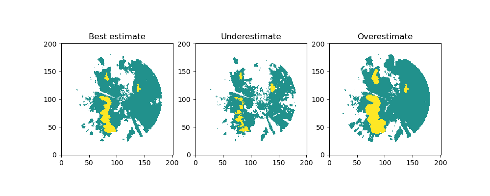
In addition to the default convective-stratiform classification, the function also returns an underestimate
(convsf_under) and an overestimate (convsf_over) to take into consideration the uncertainty when choosing
classification parameters. The under and overestimate use the same parameters, but vary the input field by a
certain value (default is 5 dBZ, can be changed with estimate_offset). The estimation can be turned off (
estimate_flag=False), but we recommend keeping it turned on.
# mask weak echo and no surface echo
convsf_masked = np.ma.masked_equal(convsf_dict["feature_detection"]["data"], 0)
convsf_masked = np.ma.masked_equal(convsf_masked, 3)
convsf_dict["feature_detection"]["data"] = convsf_masked
# underest.
convsf_masked = np.ma.masked_equal(convsf_dict["feature_under"]["data"], 0)
convsf_masked = np.ma.masked_equal(convsf_masked, 3)
convsf_dict["feature_under"]["data"] = convsf_masked
# overest.
convsf_masked = np.ma.masked_equal(convsf_dict["feature_over"]["data"], 0)
convsf_masked = np.ma.masked_equal(convsf_masked, 3)
convsf_dict["feature_over"]["data"] = convsf_masked

# Plot each estimation
plt.figure(figsize=(10, 4))
ax1 = plt.subplot(131)
ax1.pcolormesh(
    convsf_dict["feature_detection"]["data"][0, :, :],
    vmin=0,
    vmax=2,
    cmap=plt.get_cmap("viridis", 3),
)
ax1.set_title("Best estimate")
ax1.set_aspect("equal")
ax2 = plt.subplot(132)
ax2.pcolormesh(
    convsf_dict["feature_under"]["data"][0, :, :],
    vmin=0,
    vmax=2,
    cmap=plt.get_cmap("viridis", 3),
)
ax2.set_title("Underestimate")
ax2.set_aspect("equal")
ax3 = plt.subplot(133)
ax3.pcolormesh(
    convsf_dict["feature_over"]["data"][0, :, :],
    vmin=0,
    vmax=2,
    cmap=plt.get_cmap("viridis", 3),
)
ax3.set_title("Overestimate")
ax3.set_aspect("equal")
plt.show()
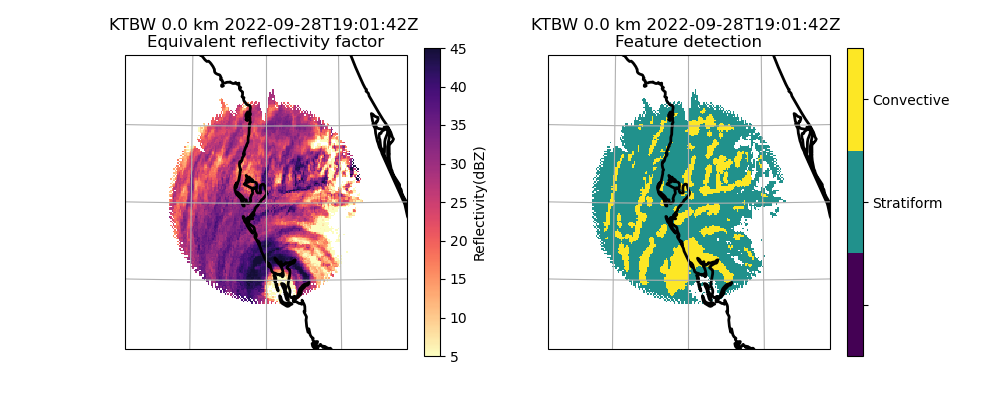
Tropical example
Let’s get a NEXRAD file from Hurricane Ian
# Read in file
nexrad_file = "s3://unidata-nexrad-level2/2022/09/28/KTBW/KTBW20220928_190142_V06"
radar = pyart.io.read_nexrad_archive(nexrad_file)

# extract the lowest sweep
radar = radar.extract_sweeps([0])

# interpolate to grid
grid = pyart.map.grid_from_radars(
    (radar,),
    grid_shape=(1, 201, 201),
    grid_limits=((0, 10000), (-200000.0, 200000.0), (-200000.0, 200000.0)),
    fields=["reflectivity"],
)

# get dx dy
dx = grid.x["data"][1] - grid.x["data"][0]
dy = grid.y["data"][1] - grid.y["data"][0]

# convective stratiform classification
convsf_dict = pyart.retrieve.conv_strat_yuter(
    grid,
    dx,
    dy,
    refl_field="reflectivity",
    always_core_thres=40,
    bkg_rad_km=20,
    use_cosine=True,
    max_diff=3,
    zero_diff_cos_val=55,
    weak_echo_thres=5,
    max_conv_rad_km=2,
    estimate_flag=False,
)

# add to grid object
# mask zero values (no surface echo)
convsf_masked = np.ma.masked_equal(convsf_dict["feature_detection"]["data"], 0)
# mask 3 values (weak echo)
convsf_masked = np.ma.masked_equal(convsf_masked, 3)
# add dimension to array to add to grid object
convsf_dict["feature_detection"]["data"] = convsf_masked
# add field
grid.add_field("convsf", convsf_dict["feature_detection"], replace_existing=True)

# create plot using GridMapDisplay
# plot variables
display = pyart.graph.GridMapDisplay(grid)
magma_r_cmap = plt.get_cmap("magma_r")
ref_cmap = mcolors.LinearSegmentedColormap.from_list(
    "ref_cmap", magma_r_cmap(np.linspace(0, 0.9, magma_r_cmap.N))
)
projection = ccrs.AlbersEqualArea(
    central_latitude=radar.latitude["data"][0],
    central_longitude=radar.longitude["data"][0],
)
# plot
plt.figure(figsize=(10, 4))
ax1 = plt.subplot(1, 2, 1, projection=projection)
display.plot_grid(
    "reflectivity",
    vmin=5,
    vmax=45,
    cmap=ref_cmap,
    transform=ccrs.PlateCarree(),
    ax=ax1,
    axislabels_flag=False,
)
ax2 = plt.subplot(1, 2, 2, projection=projection)
display.plot_grid(
    "convsf",
    vmin=0,
    vmax=2,
    cmap=plt.get_cmap("viridis", 3),
    axislabels_flag=False,
    transform=ccrs.PlateCarree(),
    ticks=[1 / 3, 1, 5 / 3],
    ticklabs=["", "Stratiform", "Convective"],
    ax=ax2,
)
plt.show()
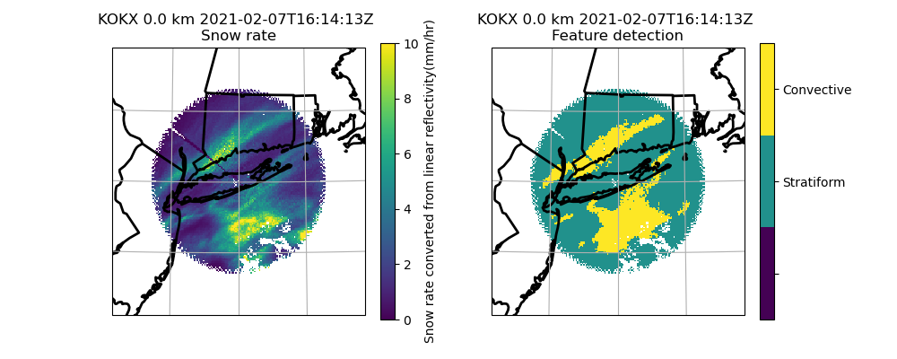
Winter storm example with image muting
Here is a final example of the convective stratiform classification using an example from a winter storm. Before doing the classification, we image mute the reflectivity to remove regions with melting or mixed precipitation. We then rescale the reflectivity to snow rate (Rasumussen et al. 2003). We recommend using a rescaled reflectivity to do the classification, but if you do make sure to changed dB_averaging to False because this parameter is used to convert reflectivity to a linear value before averaging (set dB_averaging to True for reflectivity fields in dBZ units). In this example, note how we change some of the other parameters since we are classifying snow rate instead of reflecitivity.
# Read in file
nexrad_file = "s3://unidata-nexrad-level2/2021/02/07/KOKX/KOKX20210207_161413_V06"
radar = pyart.io.read_nexrad_archive(nexrad_file)

# extract the lowest sweep
radar = radar.extract_sweeps([0])

# interpolate to grid
grid = pyart.map.grid_from_radars(
    (radar,),
    grid_shape=(1, 201, 201),
    grid_limits=((0, 10000), (-200000.0, 200000.0), (-200000.0, 200000.0)),
    fields=["reflectivity", "cross_correlation_ratio"],
)

# image mute grid object
grid = pyart.util.image_mute_radar(
    grid, "reflectivity", "cross_correlation_ratio", 0.97, 20
)

# convect non-muted reflectivity to snow rate
nonmuted_ref = grid.fields["nonmuted_reflectivity"]["data"][0, :, :]
nonmuted_ref = np.ma.masked_invalid(nonmuted_ref)

nonmuted_ref_linear = 10 ** (nonmuted_ref / 10)  # mm6/m3
snow_rate = (nonmuted_ref_linear / 57.3) ** (1 / 1.67)  #

# add to grid
snow_rate_dict = {
    "data": snow_rate[None, :, :],
    "standard_name": "snow_rate",
    "long_name": "Snow rate converted from linear reflectivity",
    "units": "mm/hr",
    "valid_min": 0,
    "valid_max": 40500,
}
grid.add_field("snow_rate", snow_rate_dict, replace_existing=True)

# get dx dy
dx = grid.x["data"][1] - grid.x["data"][0]
dy = grid.y["data"][1] - grid.y["data"][0]

# convective stratiform classification
convsf_dict = pyart.retrieve.conv_strat_yuter(
    grid,
    dx,
    dy,
    refl_field="snow_rate",
    dB_averaging=False,
    always_core_thres=4,
    bkg_rad_km=40,
    use_cosine=True,
    max_diff=1.5,
    zero_diff_cos_val=5,
    weak_echo_thres=0,
    min_dBZ_used=0,
    max_conv_rad_km=1,
    estimate_flag=False,
)

# add to grid object
# mask zero values (no surface echo)
convsf_masked = np.ma.masked_equal(convsf_dict["feature_detection"]["data"], 0)
# mask 3 values (weak echo)
convsf_masked = np.ma.masked_equal(convsf_masked, 3)
# add dimension to array to add to grid object
convsf_dict["feature_detection"]["data"] = convsf_masked
# add field
grid.add_field("convsf", convsf_dict["feature_detection"], replace_existing=True)

# create plot using GridMapDisplay
# plot variables
display = pyart.graph.GridMapDisplay(grid)
magma_r_cmap = plt.get_cmap("magma_r")
ref_cmap = mcolors.LinearSegmentedColormap.from_list(
    "ref_cmap", magma_r_cmap(np.linspace(0, 0.9, magma_r_cmap.N))
)
projection = ccrs.AlbersEqualArea(
    central_latitude=radar.latitude["data"][0],
    central_longitude=radar.longitude["data"][0],
)
# plot
plt.figure(figsize=(10, 4))
ax1 = plt.subplot(1, 2, 1, projection=projection)
display.plot_grid(
    "snow_rate",
    vmin=0,
    vmax=10,
    cmap=plt.get_cmap("viridis"),
    transform=ccrs.PlateCarree(),
    ax=ax1,
    axislabels_flag=False,
)
ax2 = plt.subplot(1, 2, 2, projection=projection)
display.plot_grid(
    "convsf",
    vmin=0,
    vmax=2,
    cmap=plt.get_cmap("viridis", 3),
    axislabels_flag=False,
    transform=ccrs.PlateCarree(),
    ticks=[1 / 3, 1, 5 / 3],
    ticklabs=["", "Stratiform", "Convective"],
    ax=ax2,
)
plt.show()
Summary of recommendations and best practices#
Tune your parameters to your specific purpose
Use a rescaled field if possible (i.e. linear reflectivity, rain or snow rate)
Keep
estimate_flag=Trueto see uncertainty in classification
References#
Steiner, M. R., R. A. Houze Jr., and S. E. Yuter, 1995: Climatological Characterization of Three-Dimensional Storm Structure from Operational Radar and Rain Gauge Data. J. Appl. Meteor., 34, 1978-2007. https://doi.org/10.1175/1520-0450(1995)034<1978:CCOTDS>2.0.CO;2.
Yuter, S. E., and R. A. Houze, Jr., 1997: Measurements of raindrop size distributions over the Pacific warm pool and implications for Z-R relations. J. Appl. Meteor., 36, 847-867. https://doi.org/10.1175/1520-0450(1997)036%3C0847:MORSDO%3E2.0.CO;2
Yuter, S. E., R. A. Houze, Jr., E. A. Smith, T. T. Wilheit, and E. Zipser, 2005: Physical characterization of tropical oceanic convection observed in KWAJEX. J. Appl. Meteor., 44, 385-415. https://doi.org/10.1175/JAM2206.1
Rasmussen, R., M. Dixon, S. Vasiloff, F. Hage, S. Knight, J. Vivekanandan, and M. Xu, 2003: Snow Nowcasting Using a Real-Time Correlation of Radar Reflectivity with Snow Gauge Accumulation. J. Appl. Meteorol. Climatol., 42, 20–36. https://doi.org/10.1175/1520-0450(2003)042%3C0020:SNUART%3E2.0.CO;2
Total running time of the script: (0 minutes 17.733 seconds)