Note
Go to the end to download the full example code.
Compare Two Radars Using Gatemapper#
Map the reflectivity field of a single radar in Antenna coordinates to another radar in Antenna coordinates and compare the fields.
print(__doc__)

# Author: Max Grover (mgrover@anl.gov) and Bobby Jackson (rjackson@anl.gov)
# License: BSD 3 clause

import warnings

import cartopy.crs as ccrs
import matplotlib.pyplot as plt
import numpy as np

import pyart
from pyart.testing import get_test_data

warnings.filterwarnings("ignore")
Read in the Data
For this example, we use two XSAPR radars from our test data.
# read in the data from both XSAPR radars
xsapr_sw_file = get_test_data("swx_20120520_0641.nc")
xsapr_se_file = get_test_data("sex_20120520_0641.nc")
radar_sw = pyart.io.read_cfradial(xsapr_sw_file)
radar_se = pyart.io.read_cfradial(xsapr_se_file)
Filter and Configure the GateMapper
We are interested in mapping the southwestern radar to the southeastern radar. Before running our gatemapper, we add a filter for only positive reflectivity values. We also need to set a distance (meters) and time (seconds) between the source and destination gate allowed for an adequate match), using the distance_tolerance/time_tolerance variables.
gatefilter = pyart.filters.GateFilter(radar_sw)
gatefilter.exclude_below("reflectivity_horizontal", 20)
gmapper = pyart.map.GateMapper(
    radar_sw,
    radar_se,
    distance_tolerance=500.0,
    time_tolerance=60,
    gatefilter_src=gatefilter,
)
radar_sw_mapped_to_radar_se = gmapper.mapped_radar(["reflectivity_horizontal"])
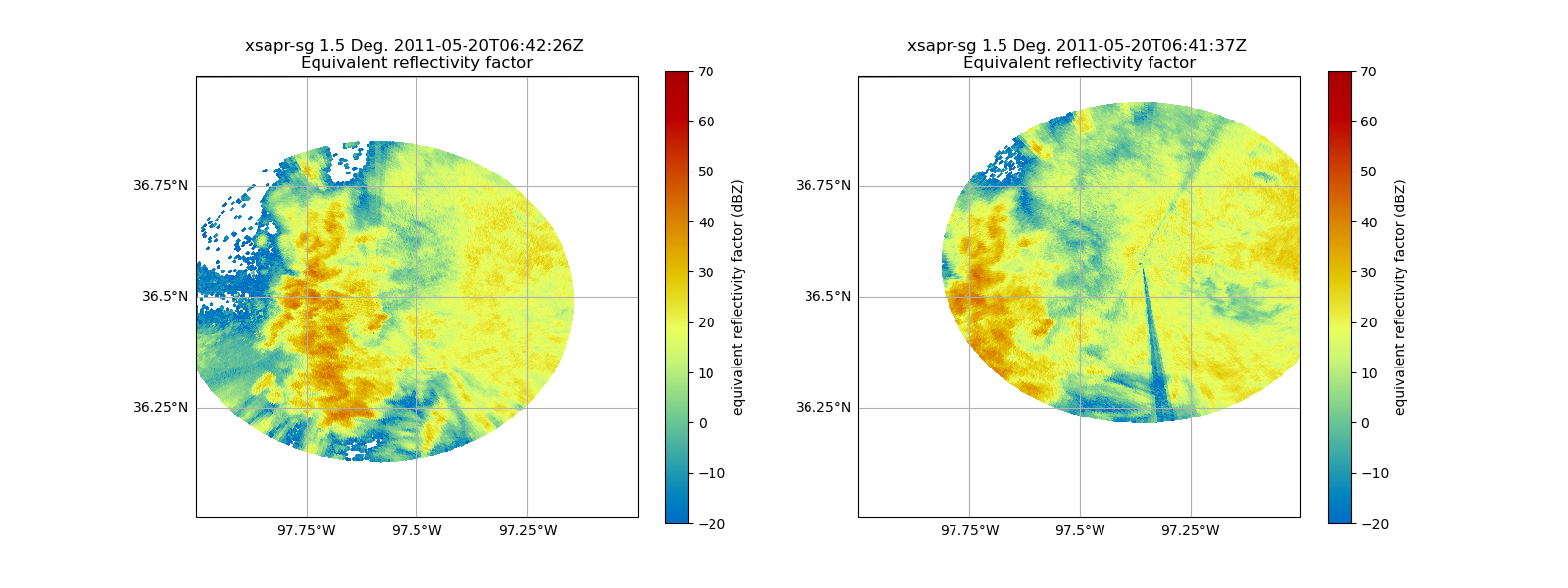
Plot the Original Data
Let’s take a look at our original fields - notice the difference in reflectivity values!
fig = plt.figure(figsize=(16, 6))
ax = plt.subplot(121, projection=ccrs.PlateCarree())

# Plot the southwestern radar
disp1 = pyart.graph.RadarMapDisplay(radar_sw)
disp1.plot_ppi_map(
    "reflectivity_horizontal",
    sweep=1,
    ax=ax,
    vmin=-20,
    vmax=70,
    min_lat=36,
    max_lat=37,
    min_lon=-98,
    max_lon=-97,
    lat_lines=np.arange(36, 37.25, 0.25),
    lon_lines=np.arange(-98, -96.75, 0.25),
)

ax2 = plt.subplot(122, projection=ccrs.PlateCarree())
disp2 = pyart.graph.RadarMapDisplay(radar_se)
disp2.plot_ppi_map(
    "reflectivity_horizontal",
    sweep=1,
    ax=ax2,
    vmin=-20,
    vmax=70,
    min_lat=36,
    max_lat=37,
    min_lon=-98,
    max_lon=-97,
    lat_lines=np.arange(36, 37.25, 0.25),
    lon_lines=np.arange(-98, -96.75, 0.25),
)
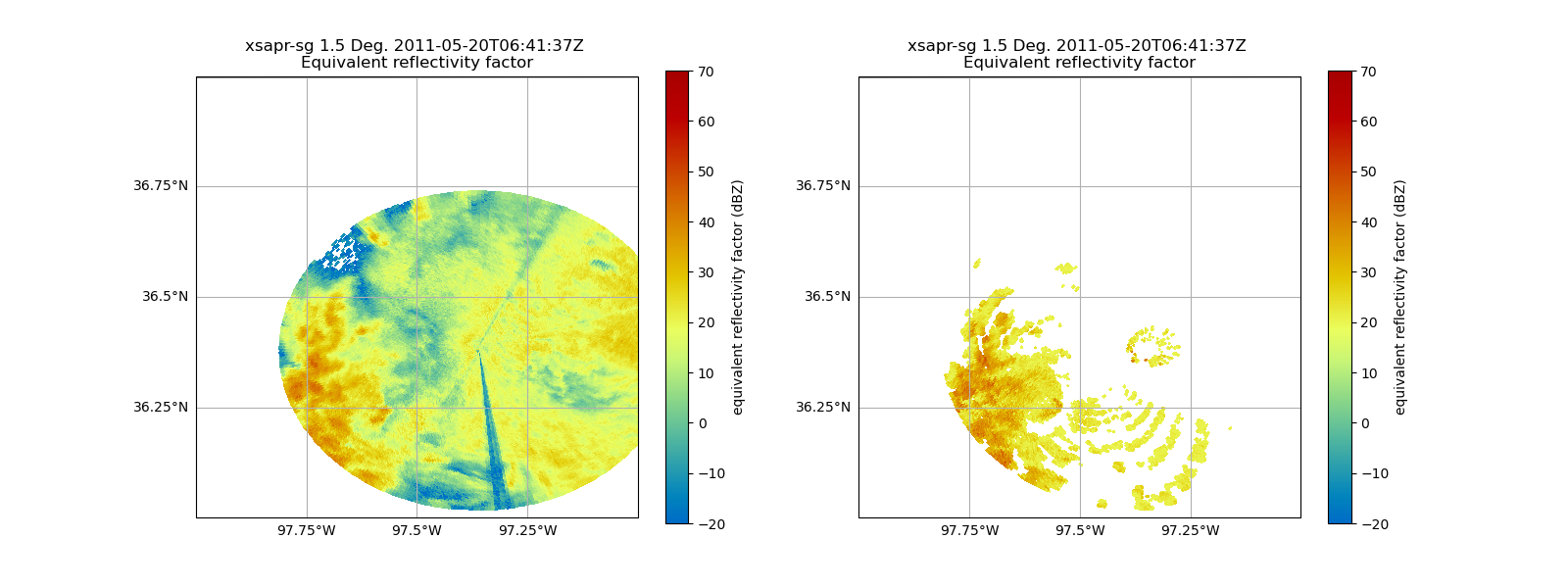
Now, we can compare our original field from the southwestern radar, to the new remapped field - there are similarities…
fig = plt.figure(figsize=(16, 6))
ax = plt.subplot(121, projection=ccrs.PlateCarree())

# Plot the southeastern radar
disp1 = pyart.graph.RadarMapDisplay(radar_se)
disp1.plot_ppi_map(
    "reflectivity_horizontal",
    sweep=1,
    ax=ax,
    vmin=-20,
    vmax=70,
    min_lat=36,
    max_lat=37,
    min_lon=-98,
    max_lon=-97,
    lat_lines=np.arange(36, 37.25, 0.25),
    lon_lines=np.arange(-98, -96.75, 0.25),
)

# Plot the southwestern radar mapped to the southeastern radar
ax2 = plt.subplot(122, projection=ccrs.PlateCarree())
disp2 = pyart.graph.RadarMapDisplay(radar_sw_mapped_to_radar_se)
disp2.plot_ppi_map(
    "reflectivity_horizontal",
    sweep=1,
    ax=ax2,
    vmin=-20,
    vmax=70,
    min_lat=36,
    max_lat=37,
    min_lon=-98,
    max_lon=-97,
    lat_lines=np.arange(36, 37.25, 0.25),
    lon_lines=np.arange(-98, -96.75, 0.25),
)
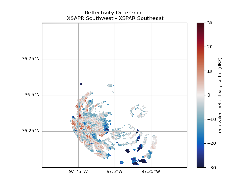
Calculate and Plot the Difference
It can be difficult to “eyeball” the difference between these two fields. Fortunately, now that our radars match coordinates, we can plot a difference. Keep in mind there is a time difference of ~ 1 minute between these plots, leading to small difference due to the precipitation moving through the domain over the course of that minute.
# Extract the numpy arrays for our reflectivity fields
reflectivity_se_radar = radar_se.fields["reflectivity_horizontal"]["data"]
reflectivity_sw_radar = radar_sw_mapped_to_radar_se.fields["reflectivity_horizontal"][
    "data"
]

# Calculate the difference between the southeastern and southwestern radar
reflectivity_difference = reflectivity_se_radar - reflectivity_sw_radar

# Add a field like this to the radar_se radar object
radar_se.add_field_like(
    "reflectivity_horizontal",
    field_name="reflectivity_bias",
    data=reflectivity_difference,
)

# Setup our figure
fig = plt.figure(figsize=(8, 6))
ax = plt.subplot(111, projection=ccrs.PlateCarree())

# Plot the difference field
disp1 = pyart.graph.RadarMapDisplay(radar_se)
disp1.plot_ppi_map(
    "reflectivity_bias",
    cmap="balance",
    title="Reflectivity Difference \n XSAPR Southwest - XSPAR Southeast",
    sweep=1,
    ax=ax,
    vmin=-30,
    vmax=30,
    min_lat=36,
    max_lat=37,
    min_lon=-98,
    max_lon=-97,
    lat_lines=np.arange(36, 37.25, 0.25),
    lon_lines=np.arange(-98, -96.75, 0.25),
)
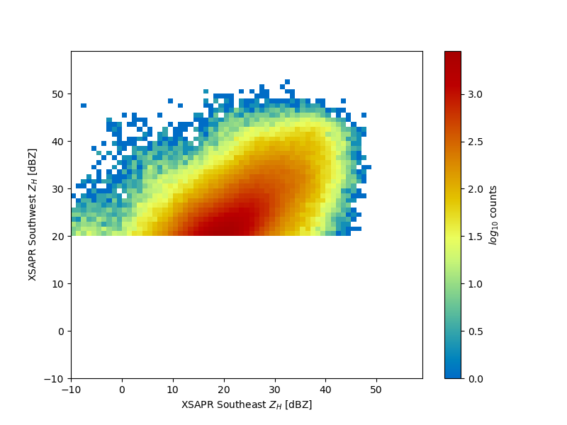
Plot a Histogram for Comparison
Another way of plotting the comparison here is using a 2-dimensional histogram,which is more helpful in this case where our scans don’t neccessarily match exactly in time.
# Include elevations above the lowest one
incl_gates = np.argwhere(radar_sw_mapped_to_radar_se.elevation["data"] > 1.0)

# Filter the reflectivity fields using the filter created above
refl_se = reflectivity_se_radar[incl_gates, :]
refl_sw = reflectivity_sw_radar[incl_gates, :]

# Make sure not include masked values
values_without_mask = np.logical_and(~refl_se.mask, ~refl_sw.mask)
refl_se = refl_se[values_without_mask]
refl_sw = refl_sw[values_without_mask]

# Set the bins for our histogram
bins = np.arange(-10, 60, 1)

# Create the 2D histogram using the flattened numpy arrays
hist = np.histogram2d(refl_se.flatten(), refl_sw.flatten(), bins=bins)[0]
hist = np.ma.masked_where(hist == 0, hist)

# Setup our figure
fig = plt.figure(figsize=(8, 6))

# Create a 1-1 comparison
x, y = np.meshgrid((bins[:-1] + bins[1:]) / 2.0, (bins[:-1] + bins[1:]) / 2.0)
c = plt.pcolormesh(x, y, np.log10(hist.T), cmap="HomeyerRainbow")

# Add a colorbar and labels
plt.colorbar(c, label="$log_{10}$ counts")
plt.xlabel("XSAPR Southeast $Z_{H}$ [dBZ]")
plt.ylabel("XSAPR Southwest $Z_{H}$ [dBZ]")

plt.show()
Total running time of the script: (0 minutes 33.642 seconds)