Dealias doppler velocities for an RHI file

In this example doppler velocities from range height indicator (RHI) scans are dealiased, using custom parameters with the region-based dealiasing algorithm in Py-ART.

print(__doc__)

# Author: Max Grover (mgrover@anl.gov)

import matplotlib.pyplot as plt
from open_radar_data import DATASETS

import pyart

# Read data from the open-radar-data package
file = DATASETS.fetch("cfrad.20211011_223602.712_to_20211011_223612.091_DOW8_RHI.nc")
radar = pyart.io.read(file)

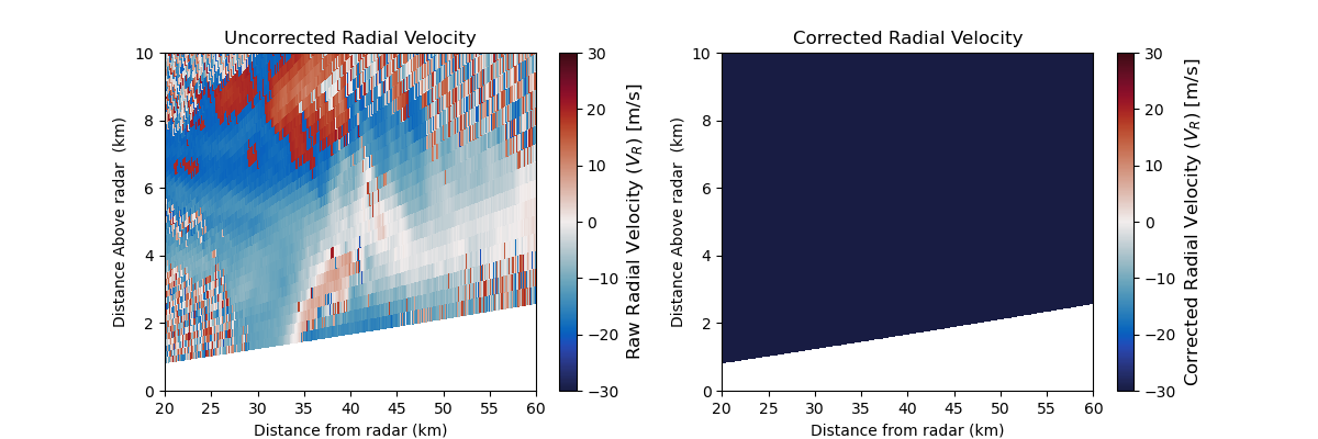
Apply the default parameters for dealiasing

Now let’s apply the default region-based technique

# Retrieve the nyquist velocity from the first sweep
nyq = radar.instrument_parameters["nyquist_velocity"]["data"][0]

# Apply the dealiasing algorithm with default parameters
velocity_dealiased = pyart.correct.dealias_region_based(
    radar,
    vel_field="VEL",
    nyquist_vel=nyq,
)

# Add the field to the radar object
radar.add_field("corrected_velocity", velocity_dealiased, replace_existing=True)

# Visualize the output
fig = plt.figure(figsize=(12, 4))
ax1 = fig.add_subplot(121)
display = pyart.graph.RadarDisplay(radar)
display.plot(
    "VEL",
    ax=ax1,
    vmin=-30,
    vmax=30,
    cmap="balance",
    title="Uncorrected Radial Velocity",
)
cbar = display.cbs[0]
# Modify the colorbar label and size
cbar.set_label(label="Raw Radial Velocity ($V_{R}$) [m/s]", fontsize=12)
plt.ylim(0, 10)
plt.xlim(20, 60)

ax2 = fig.add_subplot(122)
display = pyart.graph.RadarDisplay(radar)
display.plot(
    "corrected_velocity",
    ax=ax2,
    vmin=-30,
    vmax=30,
    cmap="balance",
    title="Corrected Radial Velocity",
)
cbar = display.cbs[0]
# Modify the colorbar label and size
cbar.set_label(label="Corrected Radial Velocity ($V_{R}$) [m/s]", fontsize=12)
plt.ylim(0, 10)
plt.xlim(20, 60)

(20.0, 60.0)

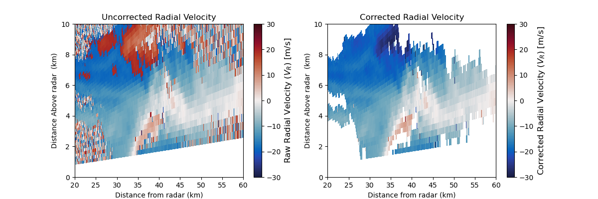
Refining the technique

If we use the default configuration, notice how extreme the values are for the output. The algorithm keys on the small variations in the clear air returns, and results in much larger values than would be expected. It is considered best practice to apply a base-level of quality control here to improve the results. We can use velocity texture as a base level, where the noisier data will be removed.

# Calculate the velocity texture and add it to the radar object
vel_texture = pyart.retrieve.calculate_velocity_texture(
    radar,
    vel_field="VEL",
    nyq=nyq,
)
radar.add_field("velocity_texture", vel_texture, replace_existing=True)

# Set up the gatefilter to be based on the velocity texture.
gatefilter = pyart.filters.GateFilter(radar)
gatefilter.exclude_above("velocity_texture", 6)

# Dealias with the gatefilter and add the corrected field to the radar object
velocity_dealiased = pyart.correct.dealias_region_based(
    radar,
    vel_field="VEL",
    nyquist_vel=nyq,
    gatefilter=gatefilter,
)
radar.add_field("corrected_velocity", velocity_dealiased, replace_existing=True)

# Visualize the output
fig = plt.figure(figsize=(12, 4))
ax1 = fig.add_subplot(121)
display = pyart.graph.RadarDisplay(radar)
display.plot(
    "VEL",
    ax=ax1,
    vmin=-30,
    vmax=30,
    cmap="balance",
    title="Uncorrected Radial Velocity",
)
cbar = display.cbs[0]

# Modify the colorbar label and size
cbar.set_label(label="Raw Radial Velocity ($V_{R}$) [m/s]", fontsize=12)
plt.ylim(0, 10)
plt.xlim(20, 60)

ax2 = fig.add_subplot(122)
display = pyart.graph.RadarDisplay(radar)
display.plot(
    "corrected_velocity",
    ax=ax2,
    vmin=-30,
    vmax=30,
    cmap="balance",
    title="Corrected Radial Velocity",
)
cbar = display.cbs[0]

# Modify the colorbar label and size
cbar.set_label(label="Corrected Radial Velocity ($V_{R}$) [m/s]", fontsize=12)
plt.ylim(0, 10)
plt.xlim(20, 60)

(20.0, 60.0)