Dealias Radial Velocities Using Xradar and Py-ART

An example which uses xradar and Py-ART to dealias radial velocities.

# Author: Max Grover (mgrover@anl.gov)
# License: BSD 3 clause


import cartopy.crs as ccrs
import matplotlib.pyplot as plt
import xradar as xd

import pyart
from pyart.testing import get_test_data

# Locate the test data and read in using xradar
filename = get_test_data("swx_20120520_0641.nc")
tree = xd.io.open_cfradial1_datatree(filename)

# Give the tree Py-ART radar methods
radar = pyart.xradar.Xradar(tree)

# Determine the nyquist velocity using the maximum radial velocity from the first sweep
nyq = radar["sweep_0"]["mean_doppler_velocity"].max().values

# Set the nyquist to what we captured above
# Calculate the velocity texture
vel_texture = pyart.retrieve.calculate_velocity_texture(
    radar, vel_field="mean_doppler_velocity", nyq=nyq
)
radar.add_field("velocity_texture", vel_texture, replace_existing=True)

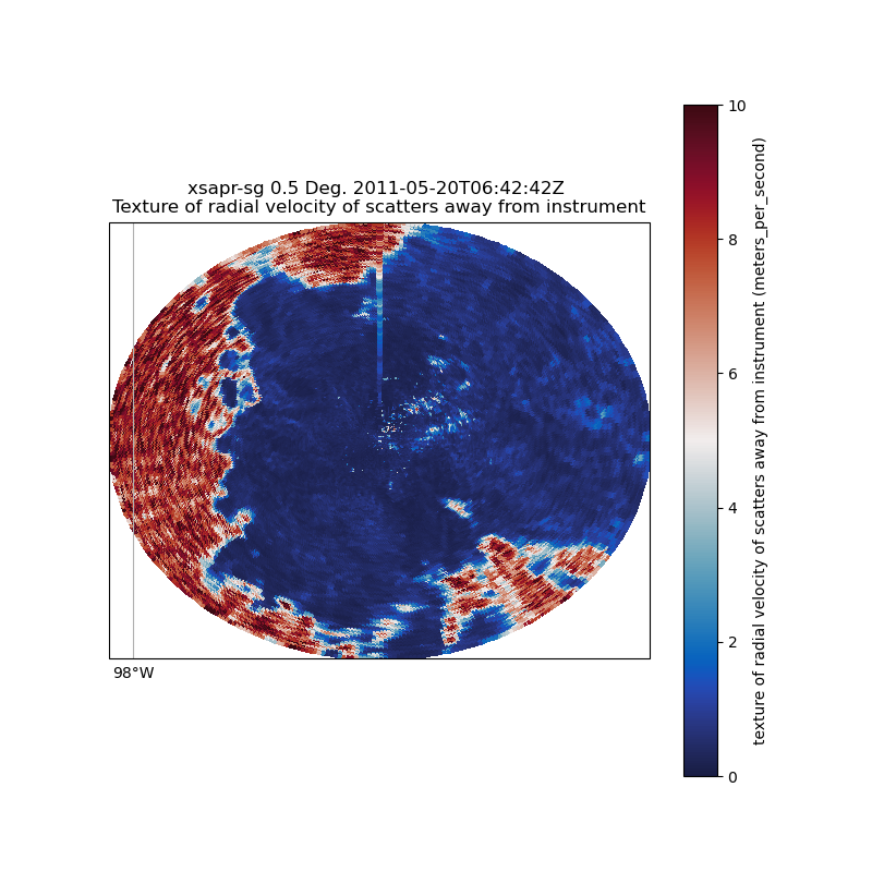
Visualize our velocity texture field Let’s use the RadarMapDisplay to visualize the texture field

fig = plt.figure(figsize=[8, 8])
display = pyart.graph.RadarMapDisplay(radar)
display.plot_ppi_map(
    "velocity_texture",
    sweep=2,
    resolution="50m",
    vmin=0,
    vmax=10,
    projection=ccrs.PlateCarree(),
    cmap="pyart_balance",
)
plt.show()

Determine a Velocity Texture Threshold Value

We can use the xradar/xarray plotting functionality here

radar["sweep_0"]["velocity_texture"].plot.hist()
plt.show()

Apply a Gatefilter Mask

We now apply this threshold, along with a reflectivity threshold, and make use of the region-based dealiasing algorithm

# Configure the gatefilter
gatefilter = pyart.filters.GateFilter(radar)
gatefilter.exclude_above("velocity_texture", 4)
gatefilter.exclude_below("corrected_reflectivity_horizontal", 0)

# At this point, we can simply used dealias_region_based to dealias the velocities
# and then add the new field to the radar.
velocity_dealiased = pyart.correct.dealias_region_based(
    radar,
    vel_field="mean_doppler_velocity",
    nyquist_vel=nyq,
    centered=True,
    gatefilter=gatefilter,
)
radar.add_field("corrected_velocity", velocity_dealiased, replace_existing=True)

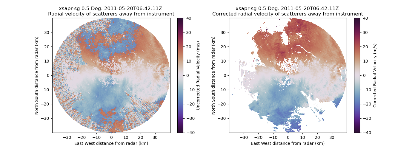
Visualize the Cleaned Radial Velocities

We can visualize the uncorrected and corrected radial velocity fields

fig = plt.figure(figsize=(14, 5))
display = pyart.graph.RadarMapDisplay(radar)
ax1 = plt.subplot(121)
display.plot_ppi(
    "mean_doppler_velocity",
    cmap="twilight_shifted",
    vmin=-40,
    vmax=40,
    colorbar_label="Uncorrected Radial Velocity (m/s)",
    ax=ax1,
)
ax2 = plt.subplot(122)
display.plot_ppi(
    "corrected_velocity",
    cmap="twilight_shifted",
    vmin=-40,
    vmax=40,
    colorbar_label="Corrected Radial Velocity (m/s)",
    ax=ax2,
)
plt.show()