Feature Detection classification

This example shows how to use the feature detection algorithm. We show how to use the algorithm to detect convective and stratiform regions in warm season events and how the algorithm can be used to detect both weak and strong features in cool-season events.

print(__doc__)

# Author: Laura Tomkins (lmtomkin@ncsu.edu)
# License: BSD 3 clause


import cartopy.crs as ccrs
import matplotlib.colors as mcolors
import matplotlib.pyplot as plt
import numpy as np
from open_radar_data import DATASETS

import pyart

How the algorithm works

The feature detection algorithm works by identifying features that exceed the background value by an amount that varies with the background value. The algorithm is heavily customizable and is designed to work with a variety of datasets. Here, we show several examples of how to use the algorithm with different types of radar data.

See Steiner et al. (1995), Yuter and Houze (1997), and Yuter et al. (2005) for full details on the algorithm. A manuscript (Tomkins et al. 2024) is in prep to describe feature detection in cool-season events (part 2).

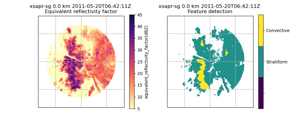
Part 1: Warm-season convective-stratiform classification

Classification of summer convective example

Our first example classifies echo from a summer convective event.

# read in file
filename = pyart.testing.get_test_data("swx_20120520_0641.nc")
radar = pyart.io.read(filename)

# extract the lowest sweep
radar = radar.extract_sweeps([0])

# interpolate to grid
grid = pyart.map.grid_from_radars(
    (radar,),
    grid_shape=(1, 201, 201),
    grid_limits=((0, 10000), (-50000.0, 50000.0), (-50000.0, 50000.0)),
    fields=["reflectivity_horizontal"],
)

# get dx dy
dx = grid.x["data"][1] - grid.x["data"][0]
dy = grid.y["data"][1] - grid.y["data"][0]

# feature detection
feature_dict = pyart.retrieve.feature_detection(
    grid,
    dx,
    dy,
    field="reflectivity_horizontal",
    always_core_thres=40,
    bkg_rad_km=20,
    use_cosine=True,
    max_diff=5,
    zero_diff_cos_val=55,
    weak_echo_thres=10,
    max_rad_km=2,
)

# add to grid object
# mask zero values (no surface echo)
feature_masked = np.ma.masked_equal(feature_dict["feature_detection"]["data"], 0)
# mask 3 values (weak echo)
feature_masked = np.ma.masked_equal(feature_masked, 3)
# add dimension to array to add to grid object
feature_dict["feature_detection"]["data"] = feature_masked
# add field
grid.add_field(
    "feature_detection", feature_dict["feature_detection"], replace_existing=True
)

# create plot using GridMapDisplay
# plot variables
display = pyart.graph.GridMapDisplay(grid)
magma_r_cmap = plt.get_cmap("magma_r")
ref_cmap = mcolors.LinearSegmentedColormap.from_list(
    "ref_cmap", magma_r_cmap(np.linspace(0, 0.9, magma_r_cmap.N))
)
projection = ccrs.AlbersEqualArea(
    central_latitude=radar.latitude["data"][0],
    central_longitude=radar.longitude["data"][0],
)

# plot
plt.figure(figsize=(10, 4))
ax1 = plt.subplot(1, 2, 1, projection=projection)
display.plot_grid(
    "reflectivity_horizontal",
    vmin=5,
    vmax=45,
    cmap=ref_cmap,
    transform=ccrs.PlateCarree(),
    ax=ax1,
)
ax2 = plt.subplot(1, 2, 2, projection=projection)
display.plot_grid(
    "feature_detection",
    vmin=0,
    vmax=2,
    cmap=plt.get_cmap("viridis", 3),
    ax=ax2,
    transform=ccrs.PlateCarree(),
    ticks=[1 / 3, 1, 5 / 3],
    ticklabs=["", "Stratiform", "Convective"],
)
plt.show()

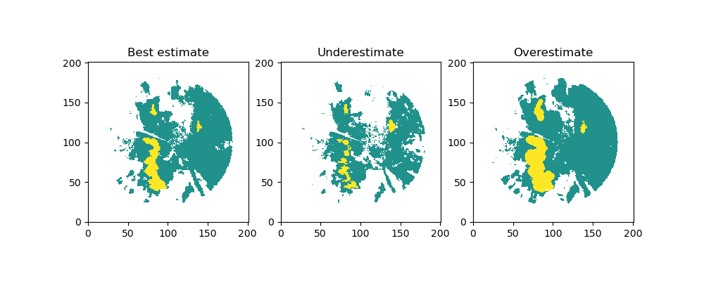
In addition to the default feature detection classification, the function also returns an underestimate (feature_under) and an overestimate (feature_over) to take into consideration the uncertainty when choosing classification parameters. The under and overestimate use the same parameters, but vary the input field by a certain value (default is 5 dBZ, can be changed with estimate_offset). The estimation can be turned off ( estimate_flag=False), but we recommend keeping it turned on.

# mask weak echo and no surface echo
feature_masked = np.ma.masked_equal(feature_dict["feature_detection"]["data"], 0)
feature_masked = np.ma.masked_equal(feature_masked, 3)
feature_dict["feature_detection"]["data"] = feature_masked
# underest.
feature_masked = np.ma.masked_equal(feature_dict["feature_under"]["data"], 0)
feature_masked = np.ma.masked_equal(feature_masked, 3)
feature_dict["feature_under"]["data"] = feature_masked
# overest.
feature_masked = np.ma.masked_equal(feature_dict["feature_over"]["data"], 0)
feature_masked = np.ma.masked_equal(feature_masked, 3)
feature_dict["feature_over"]["data"] = feature_masked

# Plot each estimation
plt.figure(figsize=(10, 4))
ax1 = plt.subplot(131)
ax1.pcolormesh(
    feature_dict["feature_detection"]["data"][0, :, :],
    vmin=0,
    vmax=2,
    cmap=plt.get_cmap("viridis", 3),
)
ax1.set_title("Best estimate")
ax1.set_aspect("equal")
ax2 = plt.subplot(132)
ax2.pcolormesh(
    feature_dict["feature_under"]["data"][0, :, :],
    vmin=0,
    vmax=2,
    cmap=plt.get_cmap("viridis", 3),
)
ax2.set_title("Underestimate")
ax2.set_aspect("equal")
ax3 = plt.subplot(133)
ax3.pcolormesh(
    feature_dict["feature_over"]["data"][0, :, :],
    vmin=0,
    vmax=2,
    cmap=plt.get_cmap("viridis", 3),
)
ax3.set_title("Overestimate")
ax3.set_aspect("equal")
plt.show()

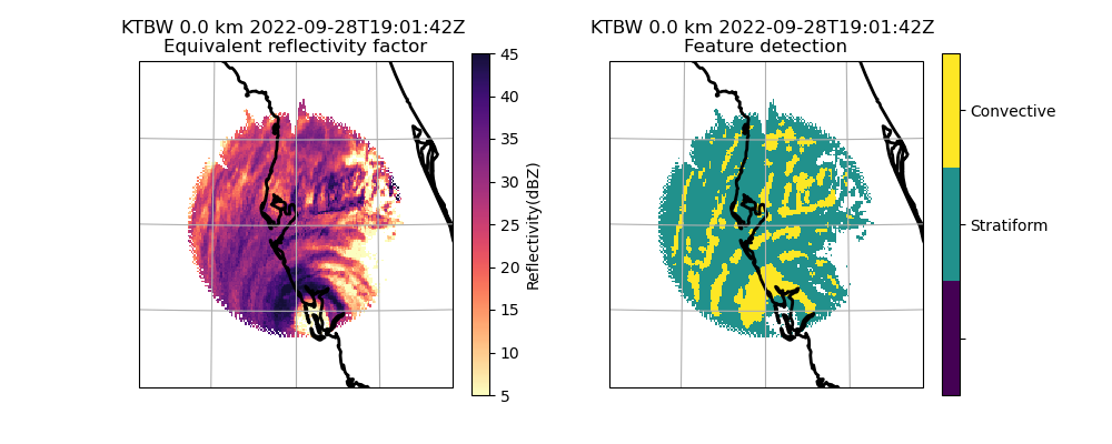
Tropical example

Let’s get a NEXRAD file from Hurricane Ian

# Read in file
nexrad_file = "s3://noaa-nexrad-level2/2022/09/28/KTBW/KTBW20220928_190142_V06"
radar = pyart.io.read_nexrad_archive(nexrad_file)

# extract the lowest sweep
radar = radar.extract_sweeps([0])

# interpolate to grid
grid = pyart.map.grid_from_radars(
    (radar,),
    grid_shape=(1, 201, 201),
    grid_limits=((0, 10000), (-200000.0, 200000.0), (-200000.0, 200000.0)),
    fields=["reflectivity"],
)

# get dx dy
dx = grid.x["data"][1] - grid.x["data"][0]
dy = grid.y["data"][1] - grid.y["data"][0]

# feature detection
feature_dict = pyart.retrieve.feature_detection(
    grid,
    dx,
    dy,
    field="reflectivity",
    always_core_thres=40,
    bkg_rad_km=20,
    use_cosine=True,
    max_diff=3,
    zero_diff_cos_val=55,
    weak_echo_thres=5,
    max_rad_km=2,
    estimate_flag=False,
)

# add to grid object
# mask zero values (no surface echo)
feature_masked = np.ma.masked_equal(feature_dict["feature_detection"]["data"], 0)
# mask 3 values (weak echo)
feature_masked = np.ma.masked_equal(feature_masked, 3)
# add dimension to array to add to grid object
feature_dict["feature_detection"]["data"] = feature_masked
# add field
grid.add_field(
    "feature_detection", feature_dict["feature_detection"], replace_existing=True
)

# create plot using GridMapDisplay
# plot variables
display = pyart.graph.GridMapDisplay(grid)
magma_r_cmap = plt.get_cmap("magma_r")
ref_cmap = mcolors.LinearSegmentedColormap.from_list(
    "ref_cmap", magma_r_cmap(np.linspace(0, 0.9, magma_r_cmap.N))
)
projection = ccrs.AlbersEqualArea(
    central_latitude=radar.latitude["data"][0],
    central_longitude=radar.longitude["data"][0],
)
# plot
plt.figure(figsize=(10, 4))
ax1 = plt.subplot(1, 2, 1, projection=projection)
display.plot_grid(
    "reflectivity",
    vmin=5,
    vmax=45,
    cmap=ref_cmap,
    transform=ccrs.PlateCarree(),
    ax=ax1,
    axislabels_flag=False,
)
ax2 = plt.subplot(1, 2, 2, projection=projection)
display.plot_grid(
    "feature_detection",
    vmin=0,
    vmax=2,
    cmap=plt.get_cmap("viridis", 3),
    axislabels_flag=False,
    transform=ccrs.PlateCarree(),
    ticks=[1 / 3, 1, 5 / 3],
    ticklabs=["", "Stratiform", "Convective"],
    ax=ax2,
)
plt.show()

Comparison with original C++ algorithm

To ensure that our algorithm here matches the original algorithm developed in C++, we compare the results from an example during the KWAJEX field campaign. The file contains the original convective-stratiform classification from the C++ algorithm. We use the algorithm implemented in Py-ART with the same settings to produce identical results.

# read in file
filename = DATASETS.fetch("convsf.19990811.221202.cdf")
grid = pyart.io.read_grid(filename)

# colormap
convsf_cmap = mcolors.LinearSegmentedColormap.from_list(
    "convsf",
    [
        (33 / 255, 145 / 255, 140 / 255),
        (253 / 255, 231 / 255, 37 / 255),
        (210 / 255, 180 / 255, 140 / 255),
    ],
    N=3,
)

# get original data from file processed in C++
x = grid.x["data"]
y = grid.y["data"]
ref = grid.fields["maxdz"]["data"][0, :, :]
csb = grid.fields["convsf"]["data"][0, :, :]
csb_masked = np.ma.masked_less_equal(csb, 0)
csl = grid.fields["convsf_lo"]["data"][0, :, :]
csl_masked = np.ma.masked_less_equal(csl, 0)
csh = grid.fields["convsf_hi"]["data"][0, :, :]
csh_masked = np.ma.masked_less_equal(csh, 0)

# plot
fig, axs = plt.subplots(2, 2, figsize=(12, 10))
# reflectivity
rpm = axs[0, 0].pcolormesh(x / 1000, y / 1000, ref, vmin=0, vmax=45, cmap="magma_r")
axs[0, 0].set_aspect("equal")
axs[0, 0].set_title("Reflectivity [dBZ]")
plt.colorbar(rpm, ax=axs[0, 0])
# convsf
csbpm = axs[0, 1].pcolormesh(
    x / 1000, y / 1000, csb_masked, vmin=1, vmax=3, cmap=convsf_cmap
)
axs[0, 1].set_aspect("equal")
axs[0, 1].set_title("convsf")
cb = plt.colorbar(csbpm, ax=axs[0, 1], ticks=[4 / 3, 2, 8 / 3])
cb.ax.set_yticklabels(["Stratiform", "Convective", "Weak Echo"])
# convsf lo
cslpm = axs[1, 0].pcolormesh(
    x / 1000, y / 1000, csl_masked, vmin=1, vmax=3, cmap=convsf_cmap
)
axs[1, 0].set_aspect("equal")
axs[1, 0].set_title("convsf lo")
cb = plt.colorbar(cslpm, ax=axs[1, 0], ticks=[])
# convsf hi
cshpm = axs[1, 1].pcolormesh(
    x / 1000, y / 1000, csh_masked, vmin=1, vmax=3, cmap=convsf_cmap
)
axs[1, 1].set_aspect("equal")
axs[1, 1].set_title("convsf hi")
cb = plt.colorbar(cshpm, ax=axs[1, 1], ticks=[4 / 3, 2, 8 / 3])
cb.ax.set_yticklabels(["Stratiform", "Convective", "Weak Echo"])
plt.show()

# now let's compare with the Python algorithm
convsf_dict = pyart.retrieve.feature_detection(
    grid,
    dx=x[1] - x[0],
    dy=y[1] - y[0],
    level_m=None,
    always_core_thres=40,
    bkg_rad_km=11,
    use_cosine=True,
    max_diff=8,
    zero_diff_cos_val=55,
    scalar_diff=None,
    use_addition=False,
    calc_thres=0,
    weak_echo_thres=15,
    min_val_used=0,
    dB_averaging=True,
    remove_small_objects=False,
    min_km2_size=None,
    val_for_max_rad=30,
    max_rad_km=5.0,
    core_val=3,
    nosfcecho=0,
    weakecho=3,
    bkgd_val=1,
    feat_val=2,
    field="maxdz",
    estimate_flag=True,
    estimate_offset=5,
)

# new data
csb_lt = convsf_dict["feature_detection"]["data"][0, :, :]
csb_lt_masked = np.ma.masked_less_equal(csb_lt, 0)
csu_lt = convsf_dict["feature_under"]["data"][0, :, :]
csu_lt_masked = np.ma.masked_less_equal(csu_lt, 0)
cso_lt = convsf_dict["feature_over"]["data"][0, :, :]
cso_lt_masked = np.ma.masked_less_equal(cso_lt, 0)

fig, axs = plt.subplots(2, 2, figsize=(12, 10))
# reflectivity
rpm = axs[0, 0].pcolormesh(x / 1000, y / 1000, ref, vmin=0, vmax=45, cmap="magma_r")
axs[0, 0].set_aspect("equal")
axs[0, 0].set_title("Reflectivity [dBZ]")
plt.colorbar(rpm, ax=axs[0, 0])
# convsf best
csbpm = axs[0, 1].pcolormesh(
    x / 1000, y / 1000, csb_lt_masked, vmin=1, vmax=3, cmap=convsf_cmap
)
axs[0, 1].set_aspect("equal")
axs[0, 1].set_title("convsf")
cb = plt.colorbar(csbpm, ax=axs[0, 1], ticks=[4 / 3, 2, 8 / 3])
cb.ax.set_yticklabels(["Stratiform", "Convective", "Weak Echo"])
# convsf under
csupm = axs[1, 0].pcolormesh(
    x / 1000, y / 1000, csu_lt_masked, vmin=1, vmax=3, cmap=convsf_cmap
)
axs[1, 0].set_aspect("equal")
axs[1, 0].set_title("convsf under")
cb = plt.colorbar(csupm, ax=axs[1, 0], ticks=[])
# convsf over
csopm = axs[1, 1].pcolormesh(
    x / 1000, y / 1000, cso_lt_masked, vmin=1, vmax=3, cmap=convsf_cmap
)
axs[1, 1].set_aspect("equal")
axs[1, 1].set_title("convsf over")
cb = plt.colorbar(csopm, ax=axs[1, 1], ticks=[4 / 3, 2, 8 / 3])
cb.ax.set_yticklabels(["Stratiform", "Convective", "Weak Echo"])
plt.show()

• 
• 

Part 2: Cool-season feature detection

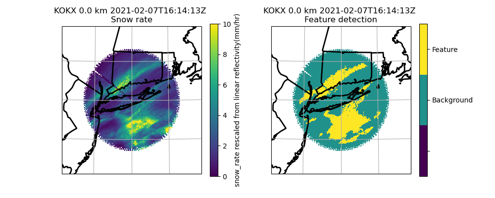
Winter storm example

In this example, we will show how to algorithm can be used to detect features (snow bands) in winter storms. Here, we rescale the reflectivity to snow rate (Rasumussen et al. 2003) in order to better represent the snow field. Note that we are not using the absolute values of the snow rate, we are only using the relative anomalies relative to the background average. We recommend using a rescaled reflectivity for this algorithm, but note that you need to change dB_averaging = False when using a rescaled field (set dB_averaging to True for reflectivity fields in dBZ units). Also note that since we are now using a snow rate field with different values, most of our parameters have changed as well.

# Read in file
nexrad_file = "s3://noaa-nexrad-level2/2021/02/07/KOKX/KOKX20210207_161413_V06"
radar = pyart.io.read_nexrad_archive(nexrad_file)

# extract the lowest sweep
radar = radar.extract_sweeps([0])

# interpolate to grid
grid = pyart.map.grid_from_radars(
    (radar,),
    grid_shape=(1, 201, 201),
    grid_limits=((0, 10000), (-200000.0, 200000.0), (-200000.0, 200000.0)),
    fields=["reflectivity", "cross_correlation_ratio"],
)

# image mute grid object
grid = pyart.util.image_mute_radar(
    grid, "reflectivity", "cross_correlation_ratio", 0.97, 20
)

# rescale reflectivity to snow rate
grid = pyart.retrieve.qpe.ZtoR(
    grid, ref_field="reflectivity", a=57.3, b=1.67, save_name="snow_rate"
)

# get dx dy
dx = grid.x["data"][1] - grid.x["data"][0]
dy = grid.y["data"][1] - grid.y["data"][0]

# feature detection
feature_dict = pyart.retrieve.feature_detection(
    grid,
    dx,
    dy,
    field="snow_rate",
    dB_averaging=False,
    always_core_thres=4,
    bkg_rad_km=40,
    use_cosine=True,
    max_diff=1.5,
    zero_diff_cos_val=5,
    weak_echo_thres=0,
    min_val_used=0,
    max_rad_km=1,
    estimate_flag=False,
)

# add to grid object
# mask zero values (no surface echo)
feature_masked = np.ma.masked_equal(feature_dict["feature_detection"]["data"], 0)
# mask 3 values (weak echo)
feature_masked = np.ma.masked_equal(feature_masked, 3)
# add dimension to array to add to grid object
feature_dict["feature_detection"]["data"] = feature_masked
# add field
grid.add_field(
    "feature_detection", feature_dict["feature_detection"], replace_existing=True
)

# create plot using GridMapDisplay
# plot variables
display = pyart.graph.GridMapDisplay(grid)

projection = ccrs.AlbersEqualArea(
    central_latitude=radar.latitude["data"][0],
    central_longitude=radar.longitude["data"][0],
)
# plot
plt.figure(figsize=(10, 4))
ax1 = plt.subplot(1, 2, 1, projection=projection)
display.plot_grid(
    "snow_rate",
    vmin=0,
    vmax=10,
    cmap=plt.get_cmap("viridis"),
    transform=ccrs.PlateCarree(),
    ax=ax1,
    axislabels_flag=False,
)
ax2 = plt.subplot(1, 2, 2, projection=projection)
display.plot_grid(
    "feature_detection",
    vmin=0,
    vmax=2,
    cmap=plt.get_cmap("viridis", 3),
    axislabels_flag=False,
    transform=ccrs.PlateCarree(),
    ticks=[1 / 3, 1, 5 / 3],
    ticklabs=["", "Background", "Feature"],
    ax=ax2,
)
plt.show()

Under and over estimate in snow

Here we show how to bound the snow rate with an under and over estimate

# get reflectivity field and copy
ref_field = grid.fields["reflectivity"]
ref_field_over = ref_field.copy()
ref_field_under = ref_field.copy()

# offset original field by +/- 2dB
ref_field_over["data"] = ref_field["data"] + 2
ref_field_under["data"] = ref_field["data"] - 2

# adjust dictionary
ref_field_over["standard_name"] = ref_field["standard_name"] + "_overest"
ref_field_over["long_name"] = ref_field["long_name"] + " overestimate"
ref_field_under["standard_name"] = ref_field["standard_name"] + "_underest"
ref_field_under["long_name"] = ref_field["long_name"] + " underestimate"

# add to grid object
grid.add_field("reflectivity_over", ref_field_over, replace_existing=True)
grid.add_field("reflectivity_under", ref_field_under, replace_existing=True)

# convert to snow rate
grid = pyart.retrieve.qpe.ZtoR(
    grid, ref_field="reflectivity_over", a=57.3, b=1.67, save_name="snow_rate_over"
)
grid = pyart.retrieve.qpe.ZtoR(
    grid, ref_field="reflectivity_under", a=57.3, b=1.67, save_name="snow_rate_under"
)

# now do feature detection with under and over estimate fields
feature_estimate_dict = pyart.retrieve.feature_detection(
    grid,
    dx,
    dy,
    field="snow_rate",
    dB_averaging=False,
    always_core_thres=4,
    bkg_rad_km=40,
    use_cosine=True,
    max_diff=1.5,
    zero_diff_cos_val=5,
    weak_echo_thres=0,
    min_val_used=0,
    max_rad_km=1,
    estimate_flag=True,
    overest_field="snow_rate_over",
    underest_field="snow_rate_under",
)

# x and y data for plotting
x = grid.x["data"]
y = grid.y["data"]

# now let's plot
fig, axs = plt.subplots(2, 2, figsize=(12, 10))
# snow rate
rpm = axs[0, 0].pcolormesh(
    x / 1000,
    y / 1000,
    grid.fields["snow_rate"]["data"][0, :, :],
    vmin=0,
    vmax=10,
)
axs[0, 0].set_aspect("equal")
axs[0, 0].set_title("Reflectivity [dBZ]")
plt.colorbar(rpm, ax=axs[0, 0])
# features best
bpm = axs[0, 1].pcolormesh(
    x / 1000,
    y / 1000,
    feature_estimate_dict["feature_detection"]["data"][0, :, :],
    vmin=0,
    vmax=3,
    cmap=plt.get_cmap("viridis", 3),
)
axs[0, 1].set_aspect("equal")
axs[0, 1].set_title("Feature detection (best)")
cb = plt.colorbar(bpm, ax=axs[0, 1], ticks=[3 / 2, 5 / 2])
cb.ax.set_yticklabels(["Background", "Feature"])
# features underestimate
upm = axs[1, 0].pcolormesh(
    x / 1000,
    y / 1000,
    feature_estimate_dict["feature_under"]["data"][0, :, :],
    vmin=0,
    vmax=3,
    cmap=plt.get_cmap("viridis", 3),
)
axs[1, 0].set_aspect("equal")
axs[1, 0].set_title("Feature detection (underestimate)")
cb = plt.colorbar(upm, ax=axs[1, 0], ticks=[3 / 2, 5 / 2])
cb.ax.set_yticklabels(["Background", "Feature"])
# features overestimate
opm = axs[1, 1].pcolormesh(
    x / 1000,
    y / 1000,
    feature_estimate_dict["feature_over"]["data"][0, :, :],
    vmin=0,
    vmax=3,
    cmap=plt.get_cmap("viridis", 3),
)
axs[1, 1].set_aspect("equal")
axs[1, 1].set_title("Feature detection (overestimate)")
cb = plt.colorbar(opm, ax=axs[1, 1], ticks=[3 / 2, 5 / 2])
cb.ax.set_yticklabels(["Background", "Feature"])
plt.show()

Strong and Faint features

We have developed a new technique which runs the algorithm twice to find features that are very distinct from the background (strong features) and features that are not very distinct from the background (faint features).

# run the algorithm again, but to find objects that are also faint
# feature detection
feature_dict = pyart.retrieve.feature_detection(
    grid,
    dx,
    dy,
    field="snow_rate",
    dB_averaging=False,
    always_core_thres=4,
    bkg_rad_km=40,
    use_cosine=False,
    scalar_diff=1.5,
    use_addition=False,
    weak_echo_thres=0,
    min_val_used=0,
    max_rad_km=1,
    estimate_flag=False,
)

# separate strong vs. faint
# mask zero values (no surface echo)
scalar_features_masked = np.ma.masked_equal(
    feature_dict["feature_detection"]["data"], 0
)
# mask 3 values (weak echo)
scalar_features_masked = np.ma.masked_equal(scalar_features_masked, 3)
# get cosine features
cosine_features_masked = grid.fields["feature_detection"]["data"]
# isolate faint features only
faint_features = scalar_features_masked - cosine_features_masked
faint_features_masked = np.ma.masked_less_equal(faint_features, 0)
# add strong and faint features
features_faint_strong = 2 * faint_features_masked.filled(
    0
) + cosine_features_masked.filled(0)
features_faint_strong_masked = np.ma.masked_where(
    cosine_features_masked.mask, features_faint_strong
)

# add to grid object
new_dict = {
    "features_faint_strong": {
        "data": features_faint_strong_masked,
        "standard_name": "features_faint_strong",
        "long name": "Faint and Strong Features",
        "valid_min": 0,
        "valid_max": 10,
        "comment_1": "3: Faint features, 2: Strong features, 1: background",
    }
}
# add field
grid.add_field(
    "features_faint_strong", new_dict["features_faint_strong"], replace_existing=True
)

# create plot using GridMapDisplay
# plot variables
display = pyart.graph.GridMapDisplay(grid)

projection = ccrs.AlbersEqualArea(
    central_latitude=radar.latitude["data"][0],
    central_longitude=radar.longitude["data"][0],
)

faint_strong_cmap = mcolors.LinearSegmentedColormap.from_list(
    "faint_strong",
    [
        (32 / 255, 144 / 255, 140 / 255),
        (254 / 255, 238 / 255, 93 / 255),
        (254 / 255, 152 / 255, 93 / 255),
    ],
    N=3,
)

# plot
plt.figure(figsize=(10, 4))
ax1 = plt.subplot(1, 2, 1, projection=projection)
display.plot_grid(
    "snow_rate",
    vmin=0,
    vmax=10,
    cmap=plt.get_cmap("viridis"),
    transform=ccrs.PlateCarree(),
    ax=ax1,
    axislabels_flag=False,
)
ax2 = plt.subplot(1, 2, 2, projection=projection)
display.plot_grid(
    "features_faint_strong",
    vmin=1,
    vmax=3,
    cmap=faint_strong_cmap,
    axislabels_flag=False,
    transform=ccrs.PlateCarree(),
    ticks=[1.33, 2, 2.66],
    ticklabs=["Background", "Strong Feature", "Faint Feature"],
    ax=ax2,
)
plt.show()

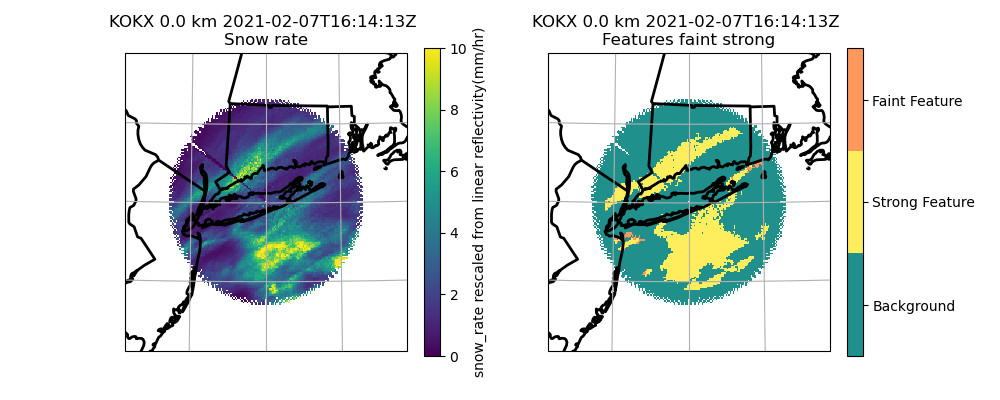
Image muted Strong and Faint features

This last section shows how we can image mute the fields (Tomkins et al. 2022) and reduce the visual prominence of melting and mixed precipitation.

# create a function to quickly apply image muting to other fields
def quick_image_mute(field, muted_ref):
    nonmuted_field = np.ma.masked_where(~muted_ref.mask, field)
    muted_field = np.ma.masked_where(muted_ref.mask, field)

    return nonmuted_field, muted_field


# get fields
snow_rate = grid.fields["snow_rate"]["data"][0, :, :]
muted_ref = grid.fields["muted_reflectivity"]["data"][0, :, :]
features = grid.fields["features_faint_strong"]["data"][0, :, :]
x = grid.x["data"]
y = grid.y["data"]

# mute
snow_rate_nonmuted, snow_rate_muted = quick_image_mute(snow_rate, muted_ref)
features_nonmuted, features_muted = quick_image_mute(features, muted_ref)

# muted colormap
grays_cmap = plt.get_cmap("gray_r")
muted_cmap = mcolors.LinearSegmentedColormap.from_list(
    "muted_cmap", grays_cmap(np.linspace(0.2, 0.8, grays_cmap.N)), 3
)


# plot
fig, axs = plt.subplots(1, 2, figsize=(10, 4))
# snow rate
srpm = axs[0].pcolormesh(x / 1000, y / 1000, snow_rate_nonmuted, vmin=0, vmax=10)
srpmm = axs[0].pcolormesh(
    x / 1000, y / 1000, snow_rate_muted, vmin=0, vmax=10, cmap=muted_cmap
)
axs[0].set_aspect("equal")
axs[0].set_title("Snow rate [mm hr$^{-1}$]")
plt.colorbar(srpm, ax=axs[0])

# features
csbpm = axs[1].pcolormesh(
    x / 1000, y / 1000, features_nonmuted, vmin=1, vmax=3, cmap=faint_strong_cmap
)
csbpmm = axs[1].pcolormesh(
    x / 1000, y / 1000, features_muted, vmin=1, vmax=3, cmap=muted_cmap
)

axs[1].set_aspect("equal")
axs[1].set_title("Feature detection")
cb = plt.colorbar(csbpm, ax=axs[1], ticks=[1.33, 2, 2.66])
cb.ax.set_yticklabels(["Background", "Strong Feature", "Faint Feature"])

plt.show()

Summary of recommendations and best practices

• Tune your parameters to your specific purpose

• Use a rescaled field if possible (i.e. linear reflectivity, rain or snow rate)

• Keep estimate_flag=True to see uncertainty in classification

References

Steiner, M. R., R. A. Houze Jr., and S. E. Yuter, 1995: Climatological Characterization of Three-Dimensional Storm Structure from Operational Radar and Rain Gauge Data. J. Appl. Meteor., 34, 1978-2007. https://doi.org/10.1175/1520-0450(1995)034<1978:CCOTDS>2.0.CO;2.

Yuter, S. E., and R. A. Houze, Jr., 1997: Measurements of raindrop size distributions over the Pacific warm pool and implications for Z-R relations. J. Appl. Meteor., 36, 847-867. https://doi.org/10.1175/1520-0450(1997)036%3C0847:MORSDO%3E2.0.CO;2

Yuter, S. E., R. A. Houze, Jr., E. A. Smith, T. T. Wilheit, and E. Zipser, 2005: Physical characterization of tropical oceanic convection observed in KWAJEX. J. Appl. Meteor., 44, 385-415. https://doi.org/10.1175/JAM2206.1

Rasmussen, R., M. Dixon, S. Vasiloff, F. Hage, S. Knight, J. Vivekanandan, and M. Xu, 2003: Snow Nowcasting Using a Real-Time Correlation of Radar Reflectivity with Snow Gauge Accumulation. J. Appl. Meteorol. Climatol., 42, 20–36. https://doi.org/10.1175/1520-0450(2003)042%3C0020:SNUART%3E2.0.CO;2

Tomkins, L. M., Yuter, S. E., Miller, M. A., and Allen, L. R., 2022: Image muting of mixed precipitation to improve identification of regions of heavy snow in radar data. Atmos. Meas. Tech., 15, 5515–5525, https://doi.org/10.5194/amt-15-5515-2022