Reading NEXRAD Data from the AWS Cloud

Within this example, we show how you can remotely access Next Generation Weather Radar (NEXRAD) Data from Amazon Web Services and plot quick looks of the datasets.

print(__doc__)

# Author: Max Grover (mgrover@anl.gov)
# License: BSD 3 clause

import cartopy.crs as ccrs
import matplotlib.pyplot as plt

import pyart

Read NEXRAD Level 2 Data

Let’s start first with NEXRAD Level 2 data, which is ground-based radar data collected by the National Oceanic and Atmospheric Administration (NOAA), as a part of the National Weather Service ### Configure our Filepath for NEXRAD Level 2 Data We will access data from the noaa-nexrad-level2 bucket, with the data organized as:

s3://noaa-nexrad-level2/year/month/date/radarsite/{radarsite}{year}{month}{date}_{hour}{minute}{second}_V06

Where in our case, we are using a sample data file from Houston, Texas (KHGX) on March 22, 2022, at 1201:25 UTC. This means our path would look like:

aws_nexrad_level2_file = (
    "s3://noaa-nexrad-level2/2022/03/22/KHGX/KHGX20220322_120125_V06"
)

We can use the pyart.io.read_nexrad_archive module to access our data, passing in the filepath.

radar = pyart.io.read_nexrad_archive(aws_nexrad_level2_file)

Let’s take a look at a summary of what fields are available.

list(radar.fields)

['spectrum_width', 'reflectivity', 'differential_phase', 'velocity', 'cross_correlation_ratio', 'clutter_filter_power_removed', 'differential_reflectivity']

Let’s plot the reflectivity/velocity fields as a first step to investigating our dataset.

Note: the reflectivity and velocity fields are in different sweeps, so we will need to specify which sweep to plot in each plot.

fig = plt.figure(figsize=(12, 4))
display = pyart.graph.RadarMapDisplay(radar)

ax = plt.subplot(121, projection=ccrs.PlateCarree())

display.plot_ppi_map(
    "reflectivity",
    sweep=0,
    ax=ax,
    colorbar_label="Equivalent Relectivity ($Z_{e}$) \n (dBZ)",
    vmin=-20,
    vmax=60,
)

ax = plt.subplot(122, projection=ccrs.PlateCarree())

display.plot_ppi_map(
    "velocity",
    sweep=1,
    ax=ax,
    colorbar_label="Radial Velocity ($V_{r}$) \n (m/s)",
    vmin=-70,
    vmax=70,
)

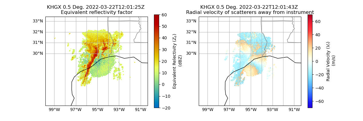
Within this plot, we see that the velocity data still has regions that are folded, indicating the dataset has not yet been dealiased.

Read NEXRAD Level 3 Data

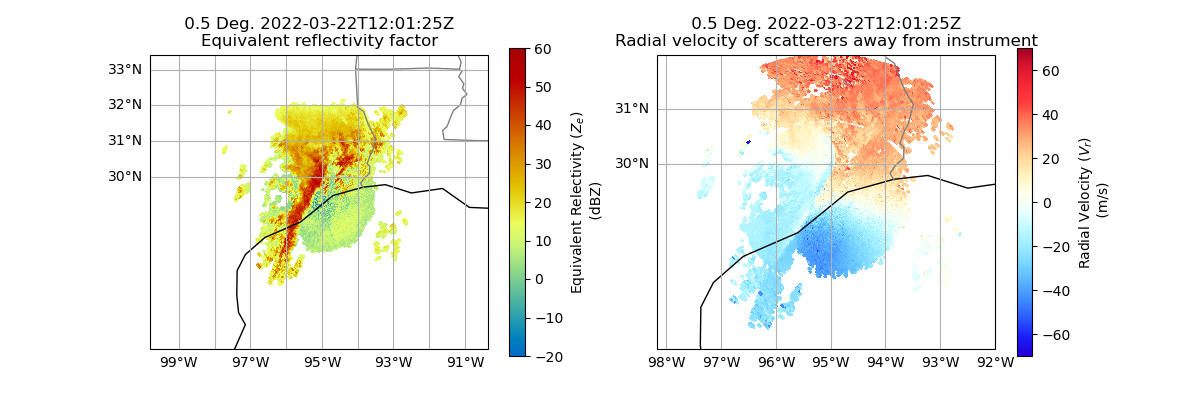
We can also access NEXRAD Level 3 data using Py-ART!

These datasets have had additional data quality processes applied, including dealiasing.

Each Level 3 data field is stored in separate file - in this example, we will look at the reflectivity and velocity field at the lowest levels. These correspond to the following variable names:

• N0U - Velocity at the lowest level

• NOQ - Reflectivity at the lowest level

These datasets are also in a different bucket (unidata-nexrad-level3), and the files are in a flat directory structure using the following naming convention:

s3://unidata-nexrad-level3/{radarsite}_{field}_{year}_{month}_{date}_{hour}_{minute}_{second}

For example, we can look at data from that same time as the NEXRAD Level 2 data used previously (March 22, 2022 at 1201 UTC)

aws_nexrad_level3_velocity_file = (
    "s3://unidata-nexrad-level3/HGX_N0U_2022_03_22_12_01_25"
)
aws_nexrad_level3_reflectivity_file = (
    "s3://unidata-nexrad-level3/HGX_N0Q_2022_03_22_12_01_25"
)

Read our Data using pyart.io.read_nexrad_level3

radar_level3_velocity = pyart.io.read_nexrad_level3(aws_nexrad_level3_velocity_file)
radar_level3_reflectivity = pyart.io.read_nexrad_level3(
    aws_nexrad_level3_reflectivity_file
)

Let’s confirm that each radar object has a single field:

print(
    "velocity radar object: ",
    list(radar_level3_velocity.fields),
    "reflectivity radar object: ",
    list(radar_level3_reflectivity.fields),
)

velocity radar object:  ['velocity'] reflectivity radar object:  ['reflectivity']

Plot a Quick Look of our NEXRAD Level 3 Data

Let’s plot the reflectivity/velocity fields as a first step to investigating our dataset.

Note: the reflectivity and velocity fields are in different radars, so we need to setup different displays.

fig = plt.figure(figsize=(12, 4))
reflectivity_display = pyart.graph.RadarMapDisplay(radar_level3_reflectivity)

ax = plt.subplot(121, projection=ccrs.PlateCarree())

reflectivity_display.plot_ppi_map(
    "reflectivity",
    ax=ax,
    colorbar_label="Equivalent Relectivity ($Z_{e}$) \n (dBZ)",
    vmin=-20,
    vmax=60,
)

velocity_display = pyart.graph.RadarMapDisplay(radar_level3_velocity)

ax = plt.subplot(122, projection=ccrs.PlateCarree())

velocity_display.plot_ppi_map(
    "velocity",
    ax=ax,
    colorbar_label="Radial Velocity ($V_{r}$) \n (m/s)",
    vmin=-70,
    vmax=70,
)