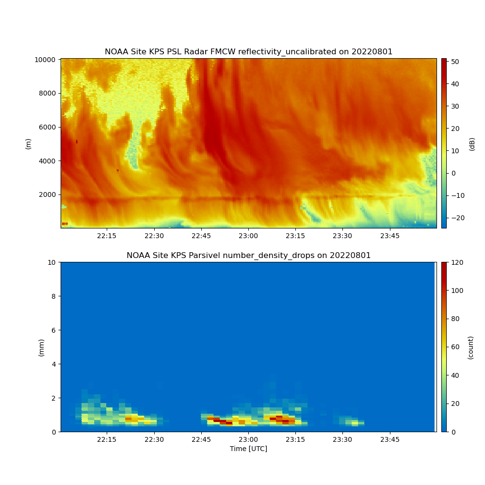
NOAA FMCW and parsivel plot

ARM and NOAA have campaigns going on in the Crested Butte, CO region and as part of that campaign NOAA has FMCW radars deployed that could benefit the broader ARM and NOAA communities. This is an example of how to plot both a NOAA FMCW PSL and NOAA parsivel two panel plot observing the same event.

Author: Zach Sherman, Adam Theisen

Downloading kps2221322.raw
Downloading kps2221323.raw

import matplotlib.pyplot as plt

import act

# Use the ACT downloader to download a file from the
# Kettle Ponds site on 8/01/2022 between 2200 and 2300 UTC.
result_22 = act.discovery.download_noaa_psl_data(
    site='kps', instrument='Radar FMCW Moment', startdate='20220801', hour='22'
)
result_23 = act.discovery.download_noaa_psl_data(
    site='kps', instrument='Radar FMCW Moment', startdate='20220801', hour='23'
)

# Read in the .raw files from both hours. Spectra data are also downloaded.
ds1 = act.io.noaapsl.read_psl_radar_fmcw_moment([result_22[-1], result_23[-1]])

# Read in the parsivel text files.
url = [
    'https://downloads.psl.noaa.gov/psd2/data/realtime/DisdrometerParsivel/Stats/kps/2022/213/kps2221322_stats.txt',
    'https://downloads.psl.noaa.gov/psd2/data/realtime/DisdrometerParsivel/Stats/kps/2022/213/kps2221323_stats.txt',
]
ds2 = act.io.noaapsl.read_psl_parsivel(url)

# Create a TimeSeriesDisplay object using both datasets.
display = act.plotting.TimeSeriesDisplay(
    {'NOAA Site KPS PSL Radar FMCW': ds1, 'NOAA Site KPS Parsivel': ds2},
    subplot_shape=(2,),
    figsize=(10, 10),
)

# Plot PSL Radar followed by the parsivel data.
display.plot(
    'reflectivity_uncalibrated',
    dsname='NOAA Site KPS PSL Radar FMCW',
    cmap='HomeyerRainbow',
    subplot_index=(0,),
)
display.plot(
    'number_density_drops',
    dsname='NOAA Site KPS Parsivel',
    cmap='HomeyerRainbow',
    subplot_index=(1,),
)
# Adjust ylims of parsivel plot.
display.axes[1].set_ylim([0, 10])
plt.show()

previous

Query and plot ASOS data

next

NEON Data