Skew-T plot of a sounding

This example shows how to make a Skew-T plot from a sounding and calculate stability indicies.

• 
• 

['base_time', 'time_offset', 'qc_time', 'pres', 'qc_pres', 'tdry', 'qc_tdry', 'dp', 'qc_dp', 'wspd', 'qc_wspd', 'deg', 'qc_deg', 'rh', 'qc_rh', 'u_wind', 'qc_u_wind', 'v_wind', 'qc_v_wind', 'wstat', 'asc', 'qc_asc', 'lat', 'lon', 'alt']
/home/runner/work/ACT/ACT/act/retrievals/sonde.py:179: UserWarning: Interpolation point out of data bounds encountered
  lfc = mpcalc.lfc(p_sorted[0], t_sorted[0], td_sorted[0])
<xarray.DataArray 'lifted_index' ()> Size: 8B
array(28.47592111)
Attributes:
    units:      kelvin
    long_name:  Lifted index

from arm_test_data import DATASETS
import xarray as xr
from matplotlib import pyplot as plt

import act

# Make sure attributes are retained
xr.set_options(keep_attrs=True)

# Read data
filename_sonde = DATASETS.fetch('sgpsondewnpnC1.b1.20190101.053200.cdf')
sonde_ds = act.io.arm.read_arm_netcdf(filename_sonde)

print(list(sonde_ds))
# Calculate stability indicies
sonde_ds = act.retrievals.calculate_stability_indicies(
    sonde_ds, temp_name='tdry', td_name='dp', p_name='pres'
)
print(sonde_ds['lifted_index'])

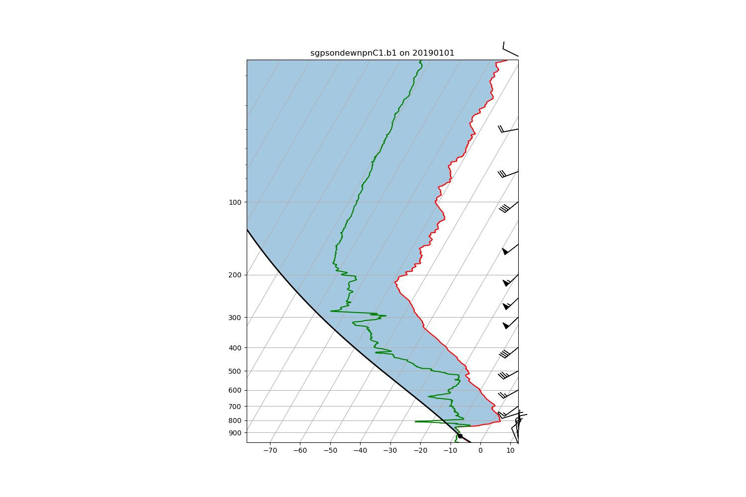
# Set up plot
skewt = act.plotting.SkewTDisplay(sonde_ds, figsize=(15, 10))

# Add data
skewt.plot_from_u_and_v('u_wind', 'v_wind', 'pres', 'tdry', 'dp')

plt.show()
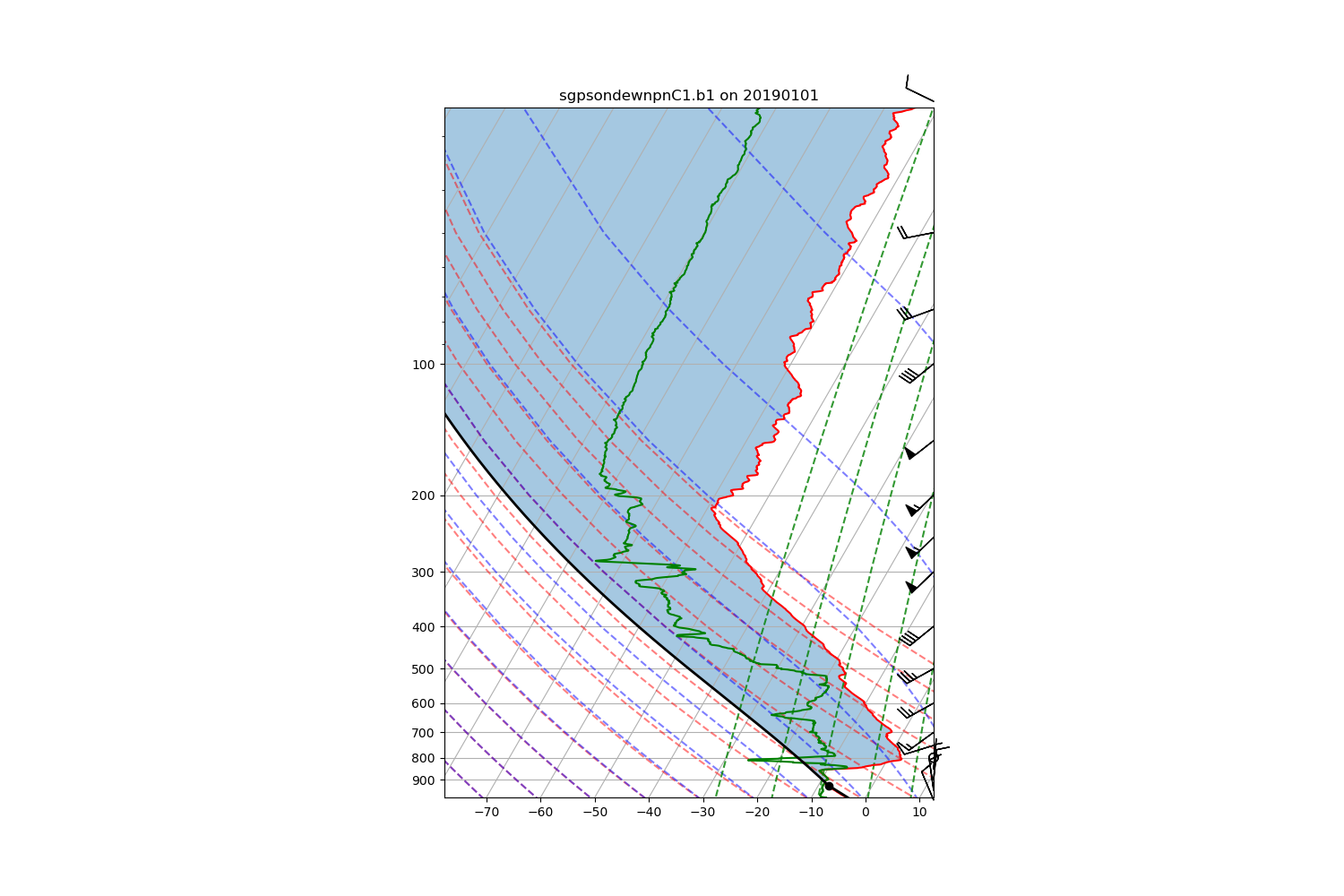
# One could also add options like adiabats and mixing lines
skewt = act.plotting.SkewTDisplay(sonde_ds, figsize=(15, 10))
skewt.plot_from_u_and_v(
    'u_wind',
    'v_wind',
    'pres',
    'tdry',
    'dp',
    plot_dry_adiabats=True,
    plot_moist_adiabats=True,
    plot_mixing_lines=True,
)
plt.show()
sonde_ds.close()

previous

Calculate and plot daily daytime temperature averages

next

Plot a timeseries of sounding data