Plotting state variables

Simple examples for plotting state variable using flag_values and flag_meanings.

Author: Ken Kehoe

• 
• 

from arm_test_data import DATASETS
from matplotlib import pyplot as plt

from act.io.arm import read_arm_netcdf
from act.plotting import TimeSeriesDisplay

# ---------------------------------------------------------------------- #
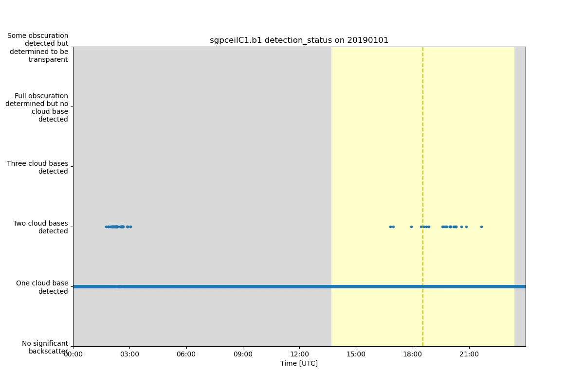
# This example will create a plot of the detection status time dimentioned
# varible and set the y axis to the string values defined in flag_meanings
# instead of plotting the flag values.
# ---------------------------------------------------------------------- #

# Read in data to plot. Only read in the variables that will be used.
variable = 'detection_status'
filename_ceil = DATASETS.fetch('sgpceilC1.b1.20190101.000000.nc')
ds = read_arm_netcdf(filename_ceil, keep_variables=[variable, 'lat', 'lon', 'alt'])

# Clean up the variable attributes to match the needed internal standard.
# Setting override_cf_flag allows the flag_meanings to be rewritten using
# the better formatted attribute values to make the plot more pretty.
ds.clean.clean_arm_state_variables(variable, override_cf_flag=True)

# Creat Plot Display by setting figure size and number of plots
display = TimeSeriesDisplay(ds, figsize=(12, 8), subplot_shape=(1,))

# Plot the variable and indicate the day/night background should be added
# to the plot.
# Since the string length for each value is long we can ask to wrap the
# text to make a better looking plot by setting the number of characters
# to keep per line with the value set to y_axis_flag_meanings. If the
# strings were short we can just use y_axis_flag_meanings=True.
display.plot(variable, day_night_background=True, y_axis_flag_meanings=18)

# Display plot in a new window
plt.show()

# ----------------------------------------------------------------------- #
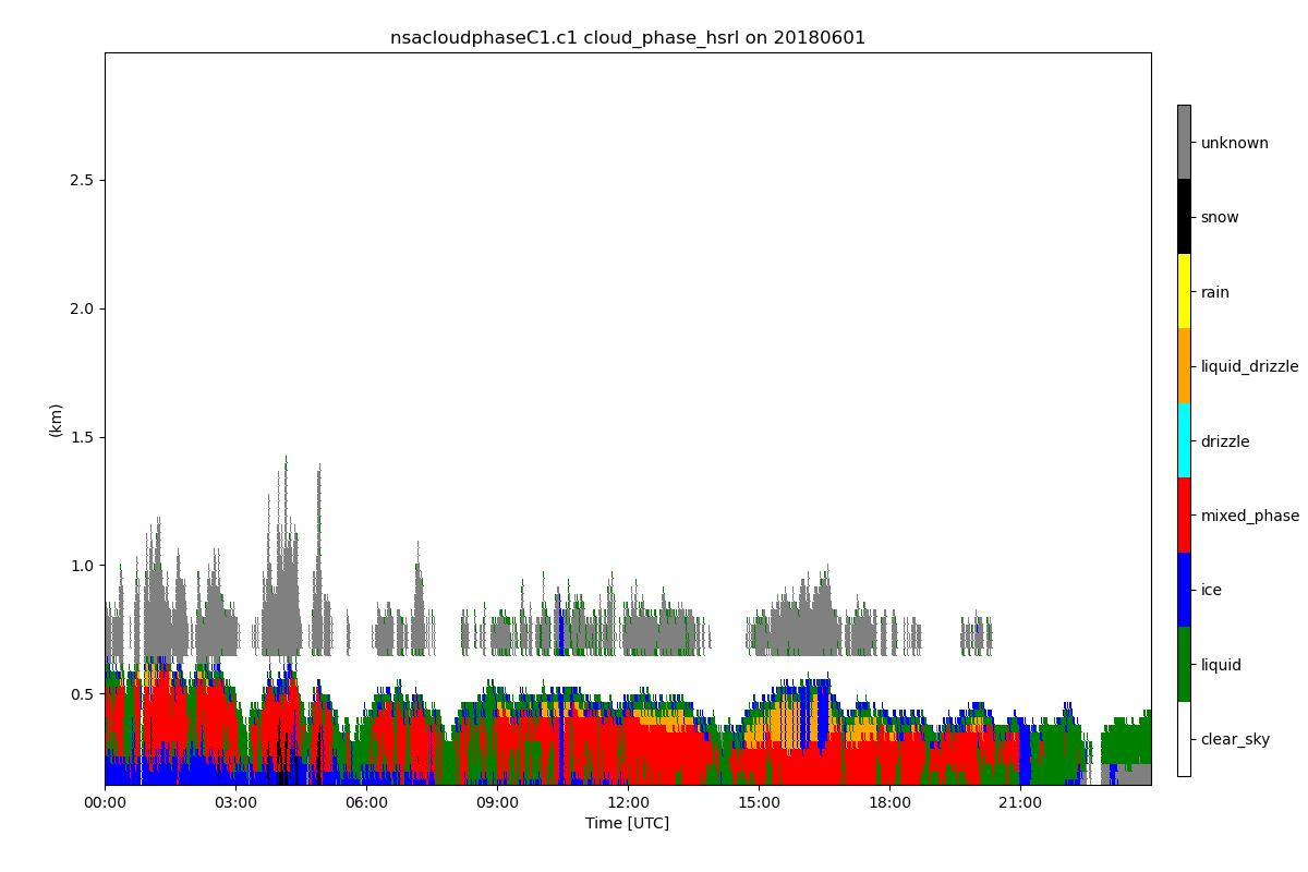
# This example will plot the 2 dimentional state variable indicating
# the cloud type classificaiton. The plot will use the correct formatting
# for x and y axis, but will show a colorbar explaining color for each value.
# ----------------------------------------------------------------------- #
# Read in data to plot. Only read in the variables that will be used.
variable = 'cloud_phase_hsrl'
filename_cloud = DATASETS.fetch('nsacloudphaseC1.c1.20180601.000000.nc')
ds = read_arm_netcdf(filename_cloud)

# Clean up the variable attributes to match the needed internal standard.
ds.clean.clean_arm_state_variables(variable, override_cf_flag=True)

# Creat Plot Display by setting figure size and number of plots
display = TimeSeriesDisplay(ds, figsize=(12, 8), subplot_shape=(1,))

# We need to pass in a dictionary containing text and color information
# for each value in the data variable. We will need to define what
# color we want plotted for each value but use the flag_values and
# flag_meanings attribute to supply the other needed information.
y_axis_labels = {}
flag_colors = ['white', 'green', 'blue', 'red', 'cyan', 'orange', 'yellow', 'black', 'gray']
for value, meaning, color in zip(
    ds[variable].attrs['flag_values'], ds[variable].attrs['flag_meanings'], flag_colors
):
    y_axis_labels[value] = {'text': meaning, 'color': color}

# Create plot and indicate the colorbar should use the defined colors
# by passing in dictionary to colorbar_lables.
# Also, since the test to display on the colorbar is longer than normal
# we can adjust the placement of the colorbar by indicating the adjustment
# of horizontal locaiton with cbar_h_adjust.
display.plot(variable, colorbar_labels=y_axis_labels, cbar_h_adjust=0)

# To provide more room for colorbar and take up more of the defined
# figure, we can adjust the margins around the initial plot.
display.fig.subplots_adjust(left=0.08, right=0.88, bottom=0.1, top=0.94)

# Display plot in a new window
plt.show()