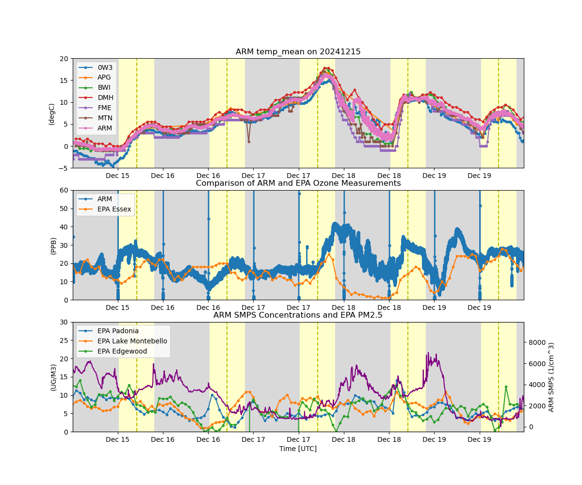
Consolidation of CoURAGE Data Sources

This example shows how to use ACT to combine multiple datasets to support ARM’s CoURAGE deployment in Baltimore, MD. Example uses ARM, EPA, and ASOS data.

Downloading: 0W3
Downloading: APG
Downloading: BWI
Downloading: DMH
Downloading: FME
Downloading: MTN
[DOWNLOADING] crgmetM1.b1.20241216.000000.cdf
[DOWNLOADING] crgmetM1.b1.20241217.000000.cdf
[DOWNLOADING] crgmetM1.b1.20241218.000000.cdf
[DOWNLOADING] crgmetM1.b1.20241219.000000.cdf
[DOWNLOADING] crgmetM1.b1.20241220.000000.cdf
[DOWNLOADING] crgmetM1.b1.20241215.000000.cdf

If you use these data to prepare a publication, please cite:

Kyrouac, J., Shi, Y., & Tuftedal, M. Surface Meteorological Instrumentation
(MET), 2024-12-15 to 2024-12-20, ARM Mobile Facility (CRG), Baltimore, MD; AMF1
(main site for CoURAGE) (M1). Atmospheric Radiation Measurement (ARM) User
Facility. https://doi.org/10.5439/1786358

[DOWNLOADING] crgaoso3S2.a1.20241216.000000.nc
[DOWNLOADING] crgaoso3S2.a1.20241217.000000.nc
[DOWNLOADING] crgaoso3S2.a1.20241215.000000.nc
[DOWNLOADING] crgaoso3S2.a1.20241219.000000.nc
[DOWNLOADING] crgaoso3S2.a1.20241218.000000.nc

If you use these data to prepare a publication, please cite:

Trojanowski, R., Springston, S., & Koontz, A. Ozone Monitor (AOSO3), 2024-12-15
to 2024-12-20, ARM Mobile Facility (CRG), Baltimore, MD; Supplemental Facility 2
in rural setting (S2). Atmospheric Radiation Measurement (ARM) User Facility.
https://doi.org/10.5439/1287329

[DOWNLOADING] crgaossmpsS2.b1.20241220.000000.nc
[DOWNLOADING] crgaossmpsS2.b1.20241218.000000.nc
[DOWNLOADING] crgaossmpsS2.b1.20241217.000000.nc
[DOWNLOADING] crgaossmpsS2.b1.20241219.000000.nc
[DOWNLOADING] crgaossmpsS2.b1.20241215.000000.nc
[DOWNLOADING] crgaossmpsS2.b1.20241216.000000.nc

If you use these data to prepare a publication, please cite:

Kuang, C., Singh, A., Howie, J., Salwen, C., & Hayes, C. Scanning mobility
particle sizer (AOSSMPS), 2024-12-15 to 2024-12-20, ARM Mobile Facility (CRG),
Baltimore, MD; Supplemental Facility 2 in rural setting (S2). Atmospheric
Radiation Measurement (ARM) User Facility. https://doi.org/10.5439/1476898

import act
from datetime import datetime
import matplotlib.pyplot as plt
import numpy as np
import os

# Get Surface Meteorology data
lat = (39.04, 39.6)
lon = (-77.10, -76.04)
time_window = [datetime(2024, 12, 15), datetime(2024, 12, 20)]
asos_dict = act.discovery.get_asos_data(time_window, lat_range=lat, lon_range=lon, regions='MD')
asos_stations = asos_dict.keys()

# Set up a dictionary to fill with data
data_dict = {}

# Fill the dictionary with ASOS data
for s in asos_stations:
    ds = asos_dict[s]
    ds = ds.where(~np.isnan(ds.tmpf), drop=True)
    ds['tmpf'].attrs['units'] = 'degF'
    ds.utils.change_units(variables='tmpf', desired_unit='degC', verbose=True)
    data_dict[s] = ds

# You need an account and token from https://docs.airnowapi.org/ first
# And then you can download EPA data
airnow_token = os.getenv('AIRNOW_API')
if airnow_token is not None and len(airnow_token) > 0:
    latlon = '-76.905,39.185,-76.158,39.499'

    ds_airnow = act.discovery.get_airnow_bounded_obs(
        airnow_token, '2024-12-15T00', '2024-12-20T23', latlon, 'OZONE,PM25', data_type='B'
    )
    ds_airnow = act.utils.convert_2d_to_1d(ds_airnow, parse='sites')
    sites = ds_airnow['sites'].values
    data_dict['EPA'] = ds_airnow
    airnow = True

# Place your username and token here
username = os.getenv('ARM_USERNAME')
token = os.getenv('ARM_PASSWORD')

# Download ARM data
if username is not None and token is not None and len(username) > 1:
    # Example to show how easy it is to download ARM data if a username/token are set
    sdate = '2024-12-15'
    edate = '2024-12-20'

    # Download and read ARM MET data
    results = act.discovery.download_arm_data(username, token, 'crgmetM1.b1', sdate, edate)
    ds_arm = act.io.arm.read_arm_netcdf(results)
    data_dict['ARM'] = ds_arm

    # Download and read ARM Ozone data
    results = act.discovery.download_arm_data(username, token, 'crgaoso3S2.a1', sdate, edate)
    ds_o3 = act.io.arm.read_arm_netcdf(results, cleanup_qc=True)
    ds_o3.qcfilter.datafilter('o3', rm_assessments=['Suspect', 'Bad'], del_qc_var=False)
    data_dict['ARM_O3'] = ds_o3

    # Download and read ARM SMPS data
    results = act.discovery.download_arm_data(username, token, 'crgaossmpsS2.b1', sdate, edate)
    ds_smps = act.io.arm.read_arm_netcdf(results)
    data_dict['ARM_SMPS'] = ds_smps

    # Set up plot and plot all surface temperature data
    display = act.plotting.TimeSeriesDisplay(data_dict, figsize=(12, 10), subplot_shape=(3,))
    for k in data_dict.keys():
        if 'ARM' not in k and k != 'EPA':
            display.plot('tmpf', dsname=k, label=k, subplot_index=(0,))
        elif k == 'ARM':
            display.plot('temp_mean', dsname=k, label=k, subplot_index=(0,))
            display.day_night_background(dsname='ARM', subplot_index=(0,))

    display.set_yrng([-5, 20], subplot_index=(0,))

    # Plot up ozone data
    title = 'Comparison of ARM and EPA Ozone Measurements'
    display.plot('o3', dsname='ARM_O3', label='ARM', subplot_index=(1,))
    if airnow:
        display.plot(
            'OZONE_sites_2',
            dsname='EPA',
            label='EPA ' + sites[2],
            subplot_index=(1,),
            set_title=title,
        )
    display.set_yrng([0, 60], subplot_index=(1,))
    display.day_night_background(dsname='ARM', subplot_index=(1,))

    # Plot SMPS data
    title = 'ARM SMPS Concentrations and EPA PM2.5'
    if airnow:
        display.plot('PM2.5_sites_0', dsname='EPA', label='EPA ' + sites[0], subplot_index=(2,))
        display.plot('PM2.5_sites_1', dsname='EPA', label='EPA ' + sites[1], subplot_index=(2,))
        display.plot(
            'PM2.5_sites_3',
            dsname='EPA',
            label='EPA ' + sites[3],
            subplot_index=(2,),
            set_title=title,
        )

    display.set_yrng([0, 30], subplot_index=(2,))
    plt.legend(loc=2)
    ax2 = display.axes[2].twinx()
    ax2.plot(ds_smps['time'], ds_smps['total_N_conc'], color='purple')
    ax2.set_ylabel('ARM SMPS (' + ds_smps['total_N_conc'].attrs['units'] + ')')
    display.day_night_background(dsname='ARM', subplot_index=(2,))

    plt.show()