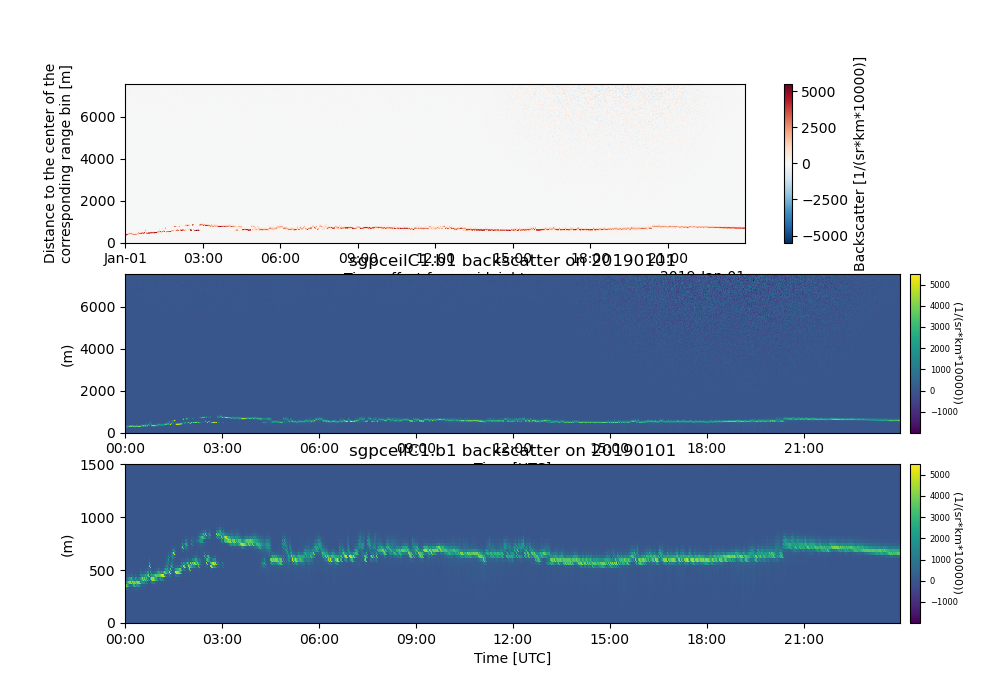
Xarray Plotting Examples

This is an example of how to use some different aspects of ACT’s plotting tools as well as Xarray’s tools.

from arm_test_data import DATASETS
import matplotlib.pyplot as plt

import act

# Set up plot space ahead of time
fig, ax = plt.subplots(3, figsize=(10, 7))

# Plotting up high-temporal resolution 2D data can be very slow at times.
# In order to increase the speed, the data can be resampled to a courser
# resolution prior to plotting.  Using Xarray's resample and selecting
# the nearest neighbor will greatly increase the speed.
filename_ceil = DATASETS.fetch('sgpceilC1.b1.20190101.000000.nc')
ds = act.io.arm.read_arm_netcdf(filename_ceil)
ds = ds.resample(time='1min').nearest()

# These data can be plotted up using the existing xarray functionality
# which is quick and easy
ds['backscatter'].plot(x='time', ax=ax[0])

# or using ACT
display = act.plotting.TimeSeriesDisplay(ds)
display.assign_to_figure_axis(fig, ax[1])
display.plot('backscatter')

# When using ACT, the axis object can also be manipulated using normal
# matplotlib calls for more personalized customizations
display = act.plotting.TimeSeriesDisplay(ds)
display.assign_to_figure_axis(fig, ax[2])
display.plot('backscatter')
display.axes[-1].set_ylim([0, 1500])

plt.show()

previous

Calculate and View Aerosol Percentages

next

Multidimensional cross sections