Working with netCDF groups

This is an example about how to work with netCDF groups. Xarray does not natively read netCDF group files, but it does have the ability to read the data with a few independent calls.

Author: Ken Kehoe

• 
• 

import xarray as xr
import matplotlib.pyplot as plt
import numpy as np
from arm_test_data import DATASETS
from act.io.arm import read_arm_netcdf
from act.plotting import TimeSeriesDisplay


# This data file is a bit complicated with the group organization. Each group
# will need to be treated as a different netCDF file for reading. We can read each group
# independently and merge into a single Dataset to use with standard Xarray or ACT methods.

# Top Level:
# data
#
# Groups:
# - data
#   - light_absorption
#     - instrument
#   - particle_concentration
#     - instrument
#   - light_scattering
#     - instrument

filename = DATASETS.fetch(
    'ESRL-GMD-AEROSOL_v1.0_HOUR_MLO_s20200101T000000Z_e20210101T000000Z_c20210214T053835Z.nc'
)

# We start by reading the location information from the top level of the netCDF file.
# This is a standard Xarary call without a group keyword. Only the top level data is read.
# The returned Dataset will contain all top level variables and top level global attributes.
# We will use the direct Xarray call to read data since there is no time dimension at the top
# level so we don't need ACT to do anything for us.
ds_location = xr.open_mfdataset(filename)

# Second, we read the 'data' group. This has a time dimension so we can use ACT to manage
# correctly reading and formatting that information. We need to specify the 'data' group
# to be read. This will read the data group but not the sub-group.
ds_data = read_arm_netcdf(filename, group='data')

# Third, we read the 'light_scattering' sub-group. We can read sub-groups
# by using standard Linux directory path notation. Notice the light_scattering group is a
# sub-group to 'data'.
ds_ls = xr.open_mfdataset(filename, group='data/light_scattering')

# We can also read the third group 'instrument'. This only contains a small amount of information
# about the instrument used to collect the data for 'light_scattering' and has no
# dimensions, only scalar values.
ds = xr.open_mfdataset(filename, group='data/light_scattering/instrument')

# Since the dimensionality aligns we can merge the three Datasets into a single Dataset.
ds = xr.merge([ds_data, ds_ls, ds_location])

# Since the data file contains data for a full year we can subset the Dataset to be easier
# to work with and process faster.
ds = ds.sel(time=slice('2020-01-01T00:00:00', '2020-01-04T23:59:59'))

# The data is written with dimensionality in reverse order from what ACT expects. We need to
# reverse the dimensionality order.
ds = ds.transpose()

# Since we want to only plot the data from one of the cut sizes we can subset the Dataset
# to only have data where the cut_size variable is set to a single value. This will reduce
# the dimensionality from 3 to 2 or 2 to 1 dimensions on the variables. Take note that
# the value of cut size is not the um value, it is the index. Since the index values
# are 0 or 1, 0 = 1 um and 1 = 10 um. We are subsetting for less than 10 um.
ds = ds.isel(cut_size=1)

# netCDF has a default _FillValue that is used to indicate when the values are missing. There
# is a known issue with float precision that does not correctly set the _FillValue to NaN
# when reading. We need to set the obviously incorrect values to NaN for the data variables
# that can have this problem.
for var_name in ds.data_vars:
    try:
        data = ds[var_name].values
        data[ds[var_name].values >= 9e36] = np.nan
        ds[var_name].values = data
    except np._core._exceptions._UFuncNoLoopError:
        pass

# This is a querk of reading the data. If we want to plot the day/night background correctly
# we need to delete these global attribute.
del ds.attrs['_file_dates']
del ds.attrs['_file_times']

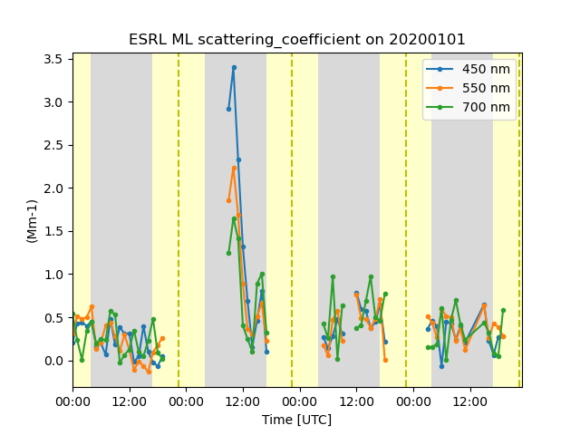
# Since the data variable has a second dimension of wavelength and we want to plot each one as a
# line plot, we will pass force_line_plot=True to force the second dimension to be removed from
# the time series plot. We will want to set the labels to view on the plot by extracting the values
# from the wavelenght dimension and pass into the plotting call.
labels = [f"{int(wl)} {ds['wavelength'].attrs['units']}" for wl in ds['wavelength'].values]

display = TimeSeriesDisplay({'ESRL ML': ds})
display.plot(
    'scattering_coefficient', day_night_background=True, force_line_plot=True, labels=labels
)
plt.show()

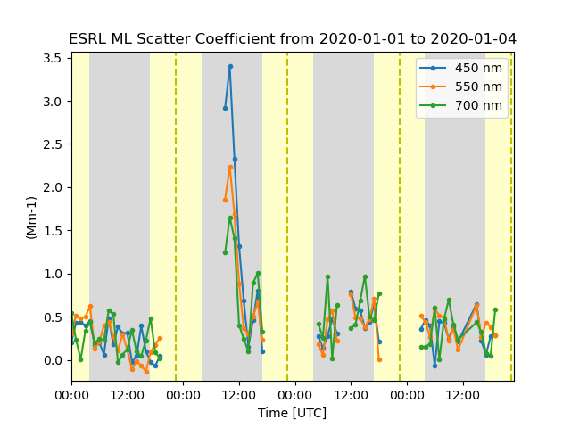
# A second option is to extract the wavelength dimension form the variable and create a new variable
# to plot. We are selecting the wavelength by using index so a value of 1 = 550 um. We need to
# provide a new variable name not already in use and correctly describes the data.
ds['scattering_coefficient_450'] = ds['scattering_coefficient'].isel(indexers={'wavelength': 0})
ds['scattering_coefficient_550'] = ds['scattering_coefficient'].isel(indexers={'wavelength': 1})
ds['scattering_coefficient_700'] = ds['scattering_coefficient'].isel(indexers={'wavelength': 2})

display = TimeSeriesDisplay({'ESRL ML': ds})
title = 'ESRL ML Scatter Coefficient from 2020-01-01 to 2020-01-04'
display.plot('scattering_coefficient_450', label=labels[0], day_night_background=True)
display.plot('scattering_coefficient_550', label=labels[1])
display.plot('scattering_coefficient_700', label=labels[2], set_title=title)
plt.show()