Plotting Baseline Surface Radiation Network (BSRN) QC Flags

Simple example for applying BSRN QC and plotting the data and the corresponding QC flags using colorblind friendly colors. https://bsrn.awi.de/data/quality-checks/

Author: Ken Kehoe

• 
• 

from arm_test_data import DATASETS
from matplotlib import pyplot as plt

import act

# Read in data and convert from ARM QC standard to CF QC standard
filename_brs = DATASETS.fetch('sgpbrsC1.b1.20190705.000000.cdf')
ds = act.io.arm.read_arm_netcdf(filename_brs, cleanup_qc=True)

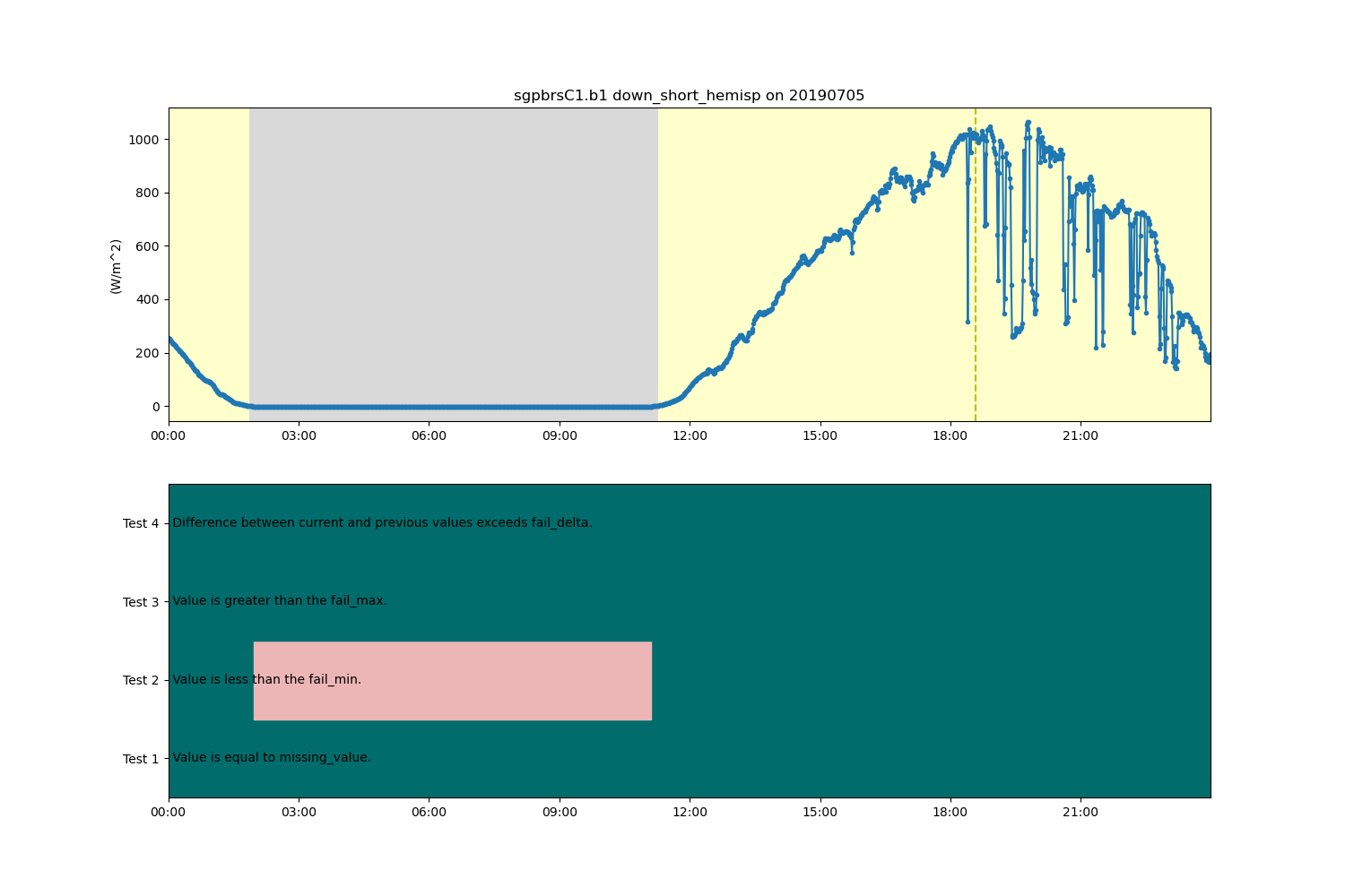
# Creat Plot Display and plot data including embedded QC from data file
variable = 'down_short_hemisp'
display = act.plotting.TimeSeriesDisplay(ds, figsize=(15, 10), subplot_shape=(2,))

# Plot radiation data in top plot
display.plot(variable, subplot_index=(0,), day_night_background=True, cvd_friendly=True)

# Plot ancillary QC data in bottom plot
display.qc_flag_block_plot(variable, subplot_index=(1,), cvd_friendly=True)
plt.show()

# Add initial BSRN QC tests to ancillary QC varialbles. Use defualts for
# test set to Physicall Possible and use_dask.
ds.qcfilter.bsrn_limits_test(
    gbl_SW_dn_name='down_short_hemisp',
    glb_diffuse_SW_dn_name='down_short_diffuse_hemisp',
    direct_normal_SW_dn_name='short_direct_normal',
    glb_SW_up_name='up_short_hemisp',
    glb_LW_dn_name='down_long_hemisp_shaded',
    glb_LW_up_name='up_long_hemisp',
)

# Add initial BSRN QC tests to ancillary QC varialbles. Use defualts for
# test set to Extremely Rare" and to use Dask processing.
ds.qcfilter.bsrn_limits_test(
    test='Extremely Rare',
    gbl_SW_dn_name='down_short_hemisp',
    glb_diffuse_SW_dn_name='down_short_diffuse_hemisp',
    direct_normal_SW_dn_name='short_direct_normal',
    glb_SW_up_name='up_short_hemisp',
    glb_LW_dn_name='down_long_hemisp_shaded',
    glb_LW_up_name='up_long_hemisp',
    use_dask=True,
)

# Add comparison BSRN QC tests to ancillary QC varialbles. Request two of the possible
# comparison tests.
ds.qcfilter.bsrn_comparison_tests(
    ['Global over Sum SW Ratio', 'Diffuse Ratio'],
    gbl_SW_dn_name='down_short_hemisp',
    glb_diffuse_SW_dn_name='down_short_diffuse_hemisp',
    direct_normal_SW_dn_name='short_direct_normal',
)

# Add K-tests QC to ancillary QC variables.
ds.qcfilter.normalized_rradiance_test(
    [
        'Clearness index',
        'Upper total transmittance',
        'Upper direct transmittance',
        'Upper diffuse transmittance',
    ],
    dni='short_direct_normal',
    dhi='down_short_hemisp',
    ghi='down_short_diffuse_hemisp',
)

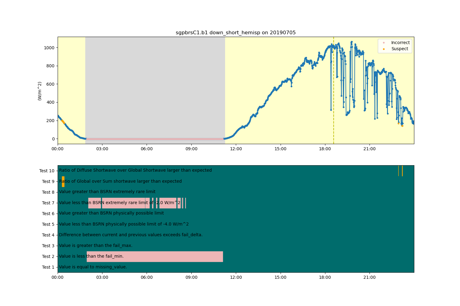
# Creat Plot Display and plot data including embedded QC from data file
variable = 'down_short_hemisp'
display = act.plotting.TimeSeriesDisplay(ds, figsize=(15, 10), subplot_shape=(2,))

# Plot radiation data in top plot. Add QC information to top plot.
display.plot(
    variable,
    subplot_index=(0,),
    day_night_background=True,
    assessment_overplot=True,
    cvd_friendly=True,
)

# Plot ancillary QC data in bottom plot
display.qc_flag_block_plot(variable, subplot_index=(1,), cvd_friendly=True)
plt.show()